Michael Elad Scientific Computing and Computational Mathematics (SCCM) Program Stanford University

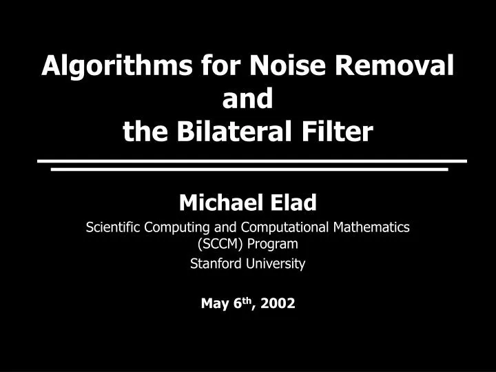
1. Algorithms for Noise Removal and the Bilateral Filter Michael Elad Scientific Computing and Computational Mathematics (SCCM) Program Stanford University May 6th, 2002

2. 1.1 General • This work deals with state-of-the-art algorithms for noise suppression. • The basic model assumption is Y=X+V where X – Unknown signal to be recovered, V – Zero-mean white Gaussian noise, Y – Measured signal.

3. White - Ideal continuous signal Red – Sampled (discrete) noisy signal 1.2 Graphically …

4. 1.3 Example

5. 1.4 Noise Suppression Noise Suppression Y X Assumptions on the noise and the desired signal X

6. 1.5 Background • There are numerous methods to suppress noise, • We are focusing on the family of methods based on • Piece-wise smoothness assumption • Maximum A-posteriori Probability Estimation (Bayesian) • State-of-the-art methods from this family: • WLS - Weighted Least Squares, • RE - Robust Estimator, • AD - Anisotropic diffusion, • Bilateral filter

7. 1.6 In Focus – Bilateral Filter • The bilateral filter was originally proposed by Tomasi and Manduchi in 1998 (ICCV) as a heuristic tool for noise removal, • A similar filter (Digital-TV) was proposed by Chan, Osher and Chen in February 2001 (IEEE Trans. On Image Proc.), • In this talk we: • Analyze the bilateral filter and relate it to the WLS/RE/AD algorithms, • Demonstrate its behavior, • Suggest further improvements to this filter.

8. Chapter 2 The WLS, RE and AD Filters

9. 2.1 MAP Based Filters • We would like the filter to produce a signal that • Is close to the measured signal, • Is smooth function, and • Preserves edges. • Using Maximum-Aposteriori-Probability formulation, we can write a penalty function which, when minimized, results with the signal we desire. • Main Question: How to formulate the above requirements?

10. 2.2 Least Squares Proximity to the measurements Spatial smoothness D- A one-sample shift operator. Thus, (X-DX) is merely a discrete one-sided derivative.

11. 2.3 Weighted Least Squares Proximity to the measurements Spatially smooth Edge Preserving by diagonal weight matrix • Based on Y: • Samples belonging to smooth regions are assigned with large weight (1). • Samples suspected of being edge points are assigned with low weight (0).

12. 2.4 WLS Solution The penalty derivative: A single SD Iteration with Y as initialization gives: What about updating the weights after each iteration ?

13. 2.5 Robust Estimation Proximity to the measurements Spatially smooth and edge preserving () - A symmetric non-negative function, e.g. ()= 2 or ()=||, etc.

14. 2.6 RE Solution The penalty derivative: A single SD Iteration with Y as initialization gives: ‘

15. ‘ For equivalence, require 2.7 WLS and RE Equivalence

16. 2.8 WLS and RE Examples The weight as a function of the derivative

17. 2.9 RE as a Bootstrap-WLS This way the RE actually applies an update of the weights after each iteration

18. 2.10 Anisotropic Diffusion • Anisotropic diffusion filter was presented originally by Perona & Malik on 1987 • The proposed filter is formulated as a Partial Differential Equation, • When discretized, the AD turns out to be the same as the Robust Estimation and the line-process techniques (see – Black and Rangarajan – 96` and Black and Sapiro – 99’).

19. 2.11 Example Original image Noisy image Var=15 WLS – 100 Iterations RE – 100 Iterations

20. Chapter 3 The Bilateral Filter

21. 3.1 General Idea • Every sample is replaced by a weighted average of its neighbors (as in the WLS), • These weights reflect two forces • How close are the neighbor and the center sample, so that larger weight to closer samples, • How similar are the neighbor and the center sample – larger weight to similar samples. • All the weights should be normalized to preserve the local mean.

22. 3.2 In an Equation Averaging over the 2N+1 neighborhood The weight The neighbor sample The result at the kth sample Normalization of the weighting Y[j] j k

23. 3.3 The Weights

24. 3.4 Graphical Example Center Sample Neighborhood It is clear that in weighting this neighborhood, we would like to preserve the step

25. 3.5 The Weights

26. 3.6 Total-Distance It appears that the weight is inversely prop. to the Total-Distance (both horizontal and vertical) from the center sample.

27. 3.7 Discrete Beltrami Flow? Total Distance This idea is similar in spirit to the ‘Beltrami Flow’ proposed by Sochen, Kimmel and Maladi (1998). There, the effective weight is the ‘Geodesic Distance’ between the samples.

28. 3.8 Kernel Properties • Per each sample, we can define a ‘Kernel’ that averages its neighborhood • This kernel changes from sample to sample! • The sum of the kernel entries is 1 due to the normalization, • The center entry in the kernel is the largest, • Subject to the above, the kernel can take any form (as opposed to filters which are monotonically decreasing).

29. 3.9 Filter Parameters As proposed by Tomasi and Manduchi, the filter is controlled by 3 parameters: N – The size of the filter support, S – The variance of the spatial distances, R – The variance of the spatial distances, and It – The filter can be applied for several iterations in order to further strengthen its edge-preserving smoothing.

30. 3.10 Additional Comments The bilateral filter is a powerful filter: • One application of it gives the effect of numerous iterations using traditional local filters, • Can work with any reasonable distances ds and dR definitions, • Easily extended to higher dimension signals, e.g. Images, video, etc. • Easily extended to vectored-signals, e.g. Color images, etc.

31. 3.11 Example Original image Noisy image Var=15 RE – 100 Iterations Bilateral (N=10, …)

32. 3.12 To Summarize Feature Bilateral filter WLS/RE/AD Behavior Edge preserve Edge preserve Support size May be large Very small Iterations Possible Must Origin Heuristic MAP-based What is the connection between the bilateral and the WLS/RE/AD filters ?

33. Chapter 4 The Bilateral Filter Origin

34. 4.1 General Idea In what follows we shall show that: • We can propose a novel penalty function {X}, extending the ones presented before, • The bilateral filter emerges as a single Jacobi iteration minimizing {X}, if Y is used for initialization, • We can get the WLS/RE filters as special cases of this more general formulation.

35. X[k]-x[k-n] 4.2 New Penalty Function Proximity to the measurements Spatially smooth and edge preservation

36. 4.3 Penalty Minimization A single Steepest-Descent iteration with Y as initialization gives

37. 4.4 Algorithm Speed-Up Instead the SD, we use a Jacobi iteration, where  is replaced by the inverse of the Hessian Matrix main diagonal Relaxation

38. 4.5 Choice of Weights Let us choose the weights in the diagonal matrix W(Y,n) as Where: (x) - Some robust function (non-negative, symmetric penalty function, e.g. (x)=|x|. V(n) - Symmetric, monotonically decreasing weight, e.g. V(n)=|n|, where 0<<1.

39. This entire operation can be viewed as a weighted average of samples in Y, where the weights themselves are dependent on Y 4.6 The Obtained Filter We can write

40. 4.7 The Filter Coefficients

41. 4.8 The Filter Properties • If we choose • we get an exact equivalence to the bilateral filter. • The values of  and  enable a control over the uniformity of the filter kernel. • The sum of all the coefficients is 1, and all are non-negative.

42. A new penalty function was defined We assumed a specific weight form We used a single Jacobi iteration We got the bilateral filter 4.9 To Recap

43. Chapter 5 ImprovingThe Bilateral Filter No time ? press HERE

44. 5.1 What can be Achieved? • Why one iteration? We can apply several iterations of the Jacobi algorithm. • Speed-up the algorithm effect by a Gauss-Siedel (GS) behavior. • Speed-up the algorithm effect by updating the output using sub-gradients. • Extend to treat piece-wise linear signals by referring to 2nd derivatives.

45. For a function of the form: The SD iteration: The Jacobi iteration: The GS iteration: The GS intuition – Compute the output sample by sample, and use the already computed values whenever possible. 5.2 GS Acceleration

46. One SD iteration: 5.3 Sub-Gradients The function we have has the form

47. 5.4 Piecewise Linear Signals Similar penalty term using 2nd derivatives for the smoothness term This way we do not penalize linear signals !

48. Chapter 6 Results

49. 6.1 General Comparison Original image Noisy image Values in the range [1,7] Gaussian Noise - =0.2 Mean-Squared-Error before the filter Noise Gain = Mean-Squared-Error after the filter

50. 6.2 Results WLS 50 iterations Gain: 3.90 RE ( ) 50 iterations Gain: 10.99 Bilateral (N=6) 1 iteration Gain: 23.50 Bilateral 10 iterations Gain: 318.90