Download
1 / 17
250 likes | 749 Views
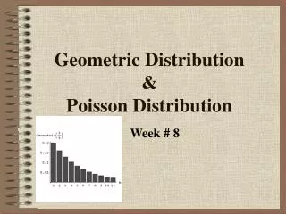
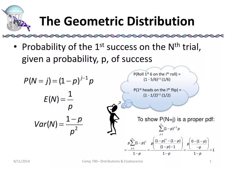
The Geometric Distribution. Probability of the 1 st success on the N th trial, given a probability, p, of success. P(Roll 1 st 6 on the i th roll) = (1 - 5/6) i-1 (1/6) P(1 st heads on the i th flip) = (1 - 1/2) i-1 (1/2). To show P(N=j) is a proper pdf:. Example.

E N D
The Geometric Distribution • Probability of the 1st success on the Nth trial, given a probability, p, of success P(Roll 1st 6 on the ith roll) = (1 - 5/6)i-1 (1/6) P(1st heads on the ith flip) = (1 - 1/2)i-1 (1/2) To show P(N=j) is a proper pdf: Comp 790– Distributions & Coalescence
Example • Difference from “Binomial” distribution • Binomial(k) = P(k successes in N trials) • Geometric(k) = P(1st success after k-1 failures) Comp 790– Distributions & Coalescence
Expected Value Proof • Expected value is value times its probability • Recall the relation: • Substituting gives: Comp 790– Distributions & Coalescence
Other Properties • Markov Property • The probability of the “next step” in a discrete or continuous process depends only on the process's present state • The process is without memory of previous events Comp 790– Distributions & Coalescence
Continuous Generalization • Geometric distributions characterize “discrete” events • Sometimes we’d like to pose questions about continuous variable, for example • Probability that a population will be inbred after T years, rather than after N generations, where T is a real number, and N is an integer • The “continuous” counterpart of the geometric distribution is the “exponential” distribution Comp 790– Distributions & Coalescence
Exponential Distribution • The Exponential density function is characterized by one parameter, a, called the “rate” or “intensity” To show Exp(a,t) is a proper pdf: Comp 790– Distributions & Coalescence
Exponential Properties • Other useful properties of U = Exp(a,t) include: • Markov property, where t2 > t1 • Assuming a second independent exponential process, V = Exp(b,t) Comp 790– Distributions & Coalescence
Approximations • The geometric distribution can be approximated with the exponential distribution in various ways • Consider the following geometric distribution • We can model discrete time as a rational fraction of of some very large number, M, that includes all intervals of interest. (i.e. 1/M, 2/M, … N/M … M/M, rather than 1, 2, 3, …) • Assuming p is small and N is large, we can approximate “continuous” time as t = j/M and a = pM There are at least “j” failures before the first success Comp 790– Distributions & Coalescence
Approximations (cont) • Recalling t = j/M and a = pM, we can rewrite (1-p)j as: • Also note, for large M: • Thus, P(T = t) = a P(N/M ≥ t) is approximately exponential with intensity a. Comp 790– Distributions & Coalescence
The Discrete-Time Coalescent • We consider the N-coalescent, or the coalescent for a sample of N genes (Kingman 1982) • N-coalescent: What is the distribution of the number of generations to find the Most Recent Common Ancestor (MCRA) for a fixed population of 2N genes • We use 2N because we recognize that the diploid case is more realistic, and it is related to the simpler haploid case by a factor of 2 Comp 790– Distributions & Coalescence
MRCA Examples Comp 790– Distributions & Coalescence
Coalescence of two genes • What is the distribution of the number of prior generations for the MCRA (waiting time)? • Probability a common parent (i.e. the MCRA is in the immediately previous generation) is: • Probability that 2 genes have a different parents is The first gene can choose its ancestor freely, but the second must choose the same of the first, thus it has 1 out of 2N choices Comp 790– Distributions & Coalescence
Going back further • Since sampling in successive generations is independent of the past, the probability that two genes find a common ancestor j generations back is: • Which is a geometric distribution with p = 1/2N • Thus, the coalescence time for 2 genes is: In the first, j-1, generations they chose different ancestors, and then in generation j they chose the same ancestor Comp 790– Distributions & Coalescence
MRCA Examples N = 10 Comp 790– Distributions & Coalescence
N-genes, no common parent • The waiting time for k ≤ 2N genes to have fewer than k lineages is: • Manipulating a little • Where, for large N, 1/N2 is negligible The 1st gene can choose it parent freely, but the next k-1 must choose from the remainder Genes without a child Comp 790– Distributions & Coalescence
N-gene Colescence • The probability k-genes have different parents is: • And one or more have a common parent: • Repeated failures for j generations leads to a geometric distribution, with Comp 790– Distributions & Coalescence
Next Time • Finish coalesence of a N-genes • The effect of approximations • The continuous-time coalescent • The effective population size Comp 790– Distributions & Coalescence