Download

1 / 64
970 likes | 3.35k Views
Hydrology Rainfall Analysis (1). Prof. Ke-Sheng Cheng Department of Bioenvironmental Systems Engineering National Taiwan UNiversity. Intensity-Duration-Frequency (IDF) Analysis . In many hydrologic design projects the first step is the determination of the rainfall event to be used.

E N D
HydrologyRainfall Analysis (1) Prof. Ke-Sheng Cheng Department of Bioenvironmental Systems Engineering National Taiwan UNiversity
Intensity-Duration-Frequency (IDF) Analysis • In many hydrologic design projects the first step is the determination of the rainfall event to be used. • The event is hypothetical, and is usually termed the design storm event. The most common approach of determining the design storm event involves a relationship between rainfall intensity (or depth), duration, and the frequency (or return period) appropriate for the facility and site location.
Steps for IDF analysis • When local rainfall data are available, IDF curves can be developed using frequency analysis. Steps for IDF analysis are: • Select a design storm duration D, say D=24 hours. • Collect the annual maximum rainfall depth of the selected duration from n years of historic data. • Determine the probability distribution of the D-hr annual maximum rainfall. The mean and standard deviation of the D-hr annual maximum rainfall are estimated.
Calculate the D-hr T-yr design storm depth XT by using the following frequency factor equation: where , and KT are mean, standard deviation and frequency factor, respectively. Note that the frequency factor is distribution-specific. • Calculate the average intensity and repeat Steps 1 through 4 for various design storm durations. • Construct the IDF curves.
Methods of plotting positions can also be used to determine the design storm depths. Most of these methods are empirical. If n is the total number of values to be plotted and m is the rank of a value in a list ordered by descending magnitude, the exceedence probability of the mth largest value, xm, is , for large n, shown in the following table.
Horner’s equation • An IDF curve is NOT a time history of rainfall within a storm. • IDF curves are often fitted to Horner's equation
Peak flow calculation-the Rational method Runoff coefficients for use in the rational formula (Table 15.1.1 of Applied Hydrology by Chow et al.)
Assumptions of the rational method • Rainfall intensity is constant at all time. • Rainfall is uniformly distributed in space. • Storm duration is equal to or longer than the time of concentration tc. • Definition of the time of concentration tc • The time for the runoff to become established and flow from the most remote part of the drainage area to drainage outlet.
Rainfall-runoff relationship associated with the rational formula
Storm Hyetographs • Hyetographs of typical storm types
Rainfall frequency analysis Design storm hyetograph Rainfall-runoff modeling Total rainfall depth Time distribution of total rainfall Runoff hydrograph The Role of A Hyetograph in Hydrologic Design
Design storm hyetograph • The SCS 24-hr design storm hyetographs
Design storm hyetographs • The alternating block model • The average rank Model • The triangular hyetograph model • The simple scaling Gauss-Markov model
The alternating block model • This model uses the intensity-duration-frequency (IDF) relationship to derive duration- and return-period-specific hyetographs (Chow et al., 1988). The hyetograph of a design storm of duration tr and return period T can be derived through the following steps:
This model does not use rainfall data of real storm events and is duration and return period specific.
The Average Rank Model • Pilgrim and Cordery (1975) developed this model by considering the average rainfall- percentages of ranked rainfalls and the average rank of each time interval within a storm. Procedures for establishment of the hyetograph model are:
The average rank model is duration-specific and requires rainfall data of storm events of the same pre-specified duration. Since storm duration varies significantly, it may be difficult to gather enough storm events of the same duration.
Raingauge Network • Minimum density of precipitation stations (WMO) • Ten percent of raingauge stations should be equipped with self-recording gauges to know the intensities of rainfall.
Adequacy of Raingauge Stations • The minimum number of raingauges N required to achieve a desired level of accuracy for the estimation of area-average rainfall can be determined by the following criteria: • the coefficient of variation approach • the statistical sampling approach
The coefficient of variation approach • If there are already some raingauge stations in a catchment, the optimal number of stations that should exist to have an assigned percentage of error in the estimation of mean rainfall is obtained by statistical analysis as:
This approach is based on the idea that the standard deviation of the estimated average rainfall should not be larger than a specified percentage of the areal average rainfall.
Weak Law of Large Numbers (WLLN) • Let f(.) be a density with mean μ and variance σ2, and let be the sample mean of a random sample of size n from f(.). Let εand δ be any two specified numbers satisfying ε>0 and 0<δ<1. If n is any integer greater than , then Dept of Bioenvironmental Systems Engineering National Taiwan University
Dept of Bioenvironmental Systems Engineering National Taiwan University
(Example) Suppose that some distribution with an unknown mean has variance equal to 1. How large a random sample must be taken in order that the probability will be at least 0.95 that the sample mean will lie within 0.5 of the population mean? Dept of Bioenvironmental Systems Engineering National Taiwan University
(Example) How large a random sample must be taken in order that you are 99% certain that is within 0.5σ of μ? Dept of Bioenvironmental Systems Engineering National Taiwan University
Raingauge network design • Assuming there are already some raingauge stations in a catchment, and we are interested in determining the optimal number of stations that should exist to achieve a desired accuracy in the estimation of mean rainfall. • Two approaches • (1) The sample standard deviation should not exceed a certain portion of the population mean. • (2) Dept of Bioenvironmental Systems Engineering National Taiwan University
Criterion 1Standard deviation of the sample mean should not exceed a certain portion of the population mean. Dept of Bioenvironmental Systems Engineering National Taiwan University
Criterion 2 • From the weak law of large numbers, Dept of Bioenvironmental Systems Engineering National Taiwan University
Preparation of data • Before using the rainfall records of a station, it is necessary to firstly check the data for continuity and consistency. • The continuity of a record may be broken with missing data due to many reasons such as damage or fault in a raingauge during a period. • Missing data can be estimated using data of neighboring stations. In these calculations thenormal rainfall is used as a standard for comparison.
The normal rainfall is the average value of rainfall at a particular date, month or year over a specified 30-year period. The 30-year normals are recomputed every decade. Thus the term normal annual precipitation at station A means the average annual precipitation at A based on a specified 30-years of record.
Test for record consistency • Some of the common causes for inconsistency of record include: • Shifting of a raingauge station to a new location, • The neighborhood of the station undergoing a marked change.
Double-mass curve technique • The checking for inconsistency of a record is done by the double-mass curve technique. This technique is based on the principle that when each recorded data comes from the same parent population, they are consistent. • A group of n (usually 5 to 10) base stations in the neighborhood of the problem station X is selected. • Annual (or monthly mean) rainfall data of station X and also the average rainfall of the group of base stations covering a long period is arranged in the reverse chronological order (i.e. the latest record as the first entry and the oldest record as the last entry in the list).
It is apparent that the more homogeneous the base station records are, the more accurate will be the corrected values at station X. A change in slope is normally taken as significant only where it persists for more than five years.
Depth-Area-Duration Curve • The technique of depth-area-duration analysis (DAD) determines primarily themaximumfalls for different durations over a range of areas. The data required for a DAD analysis are shown in the following figure.