Download
1 / 20
200 likes | 322 Views
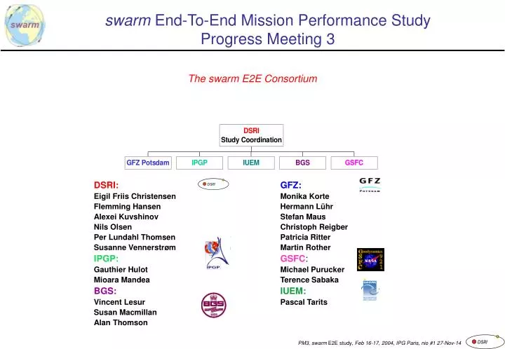
swarm End-To-End Mission Performance Study Progress Meetin g 3. DSRI: Eigil Friis Christensen Flemming Hansen Alexei Kuvshinov Nils Olsen Per Lundahl Thomsen Susanne Vennerstrøm IPGP: Gauthier Hulot Mioara Mandea BGS: Vincent Lesur Susan Macmillan Alan Thomson. GFZ: Monika Korte

E N D
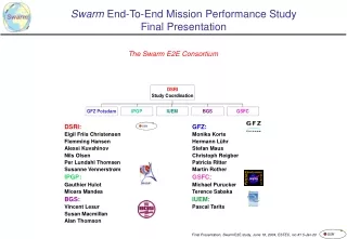
swarm End-To-End Mission Performance StudyProgress Meeting 3 DSRI: Eigil Friis Christensen Flemming Hansen Alexei Kuvshinov Nils Olsen Per Lundahl Thomsen Susanne Vennerstrøm IPGP: Gauthier Hulot Mioara Mandea BGS: Vincent Lesur Susan Macmillan Alan Thomson GFZ: Monika Korte Hermann Lühr Stefan Maus Christoph Reigber Patricia Ritter Martin Rother GSFC: Michael Purucker Terence Sabaka IUEM: Pascal Tarits The swarm E2E Consortium
Draft Agenda Working Meeting (Monday) • Presentation of preliminary results achieved in Task 3 (all) • How to proceed • General discussion Progress Meeting 3 (Tuesday) • Achieved Milestones • Plans for the remaining of Task 3 • General discussion
Achieved Milestones • Synthetic Data of Constellation #2 • Recovery of field contributions • emphasis on: • lithospheric field • secular variation • mantle conductivity • demonstration of superiority of constellation
Forward Scheme for Task 3 • Constellation #2 designed • based on experience gained with constellation #1 • consists of 6 satellites (3 high, 3 low) • up to 4 satellites will be chosen from the pool of 6 satellites • Synthetic data for constellation #2 • improved parameterization of magnetospheric sources: n=3, m=1 based on hour-by-hour analysis of world-wide distributed observatory data after removal of CM4 • induced contributions are considered using a 3D conductivity model (oceans, sediments + deep-located mantle inhomogeneities) • ”boosted” secular variation • Noise added (based on CHAMP experience and swarm specifications)
Advantage of two satellites flying side-by-side Strong attenuation of large-scale magnetospheric terms Amplification of m»0 terms
Power Spectral Density of simulated swarm noise Phase A System Simulator models produce time series of magnetic field that are off by several nT. s = (0.1, 0.07, 0.07) nT in agreement with swarm performance requirements
Highlights of Field Recovery • Recovery of Lithospheric Field (n = 100+) • Recovery of high-degree secular variation (n = 14+) • Mapping of 3D mantle conductivity
Recovering the Lithospheric FieldAccumulated Error at Ground • More than Ö2 improvement if 2nd satellite added • Adding 3rd satellite (different local time) gives improved low-degree terms • Best result by combining results from CI and filter method
Comparison of Filter Method and CI • CI superior at n<70, especially for terms m close to 0 • Filter method is superior for n > 70
CosmeticsAccumulated error at ground or at 100 km altitude? • ”More improvement” at altitudes above ground
Can we push the maximum degree? • Filter method gives correlation > 0.9 even for n=110 • Suggestion: re-do the analysis (with swarm 4+5) with a new crustal field that goes up to n=150 • preparation of new data: a few days (NIO) • test with ”clean” data (NIO) • analysis using all data sources (GFZ)
Recovery of Lithospheric Field Br at ground Synthetic crustal field up to N=149 by combination of MF3 (n<70) and a model of remanent magnetization (Purucker + Dyment) N = 60 (present case) N = 110 N = 150 -200 nT 200
Recovery of Lithospheric Field Br at 100 km altitude N = 60 (present case) N = 110 N = 150 -50 nT 50
Induction StudiesMapping of 3D Mantle Conductivity Forward conductivity model contains • near-surface conductors (oceans, sediments) • local (small-scale) inhomogeneities(plumes, subduction zones) • regional inhomogeneities(e.g., covering one plate) Attempt to map 3D mantle conductivity structure
Transfer Function: C-response • C from local Bz and BH , derived using a SHA • Frequency dependence of C(w) (or of other transfer functions) provides information on conductivity-depth structure s(z) Electromagnetic Induction:Attenuation of B with depth z:
Transfer Functions - Conductivity Models Transfer functions and their interpretation by means of conductivity models Constable & Constable, 2003
Mapping of 3D mantle structure Real and imaginary part of the local C-response for a period of 7 days, reconstructed from time-series of spherical harmonic coefficients up to N. N = 5 N = 9 N = 45 (all terms)
Mapping of 3D mantle conductivity with swarm • The presented results are based on time series of SH expansion coefficients. • Next step: to estimate these time series using swarm • Sampling rate: 12 hours (since we are interested in periods of a few days) • swarm should give sufficient data coverage to recover induced fields with N=5 or even N=9, together with inducing field (n=1-3, m=0,1) • Suggestion: • Estimation of time series from clean data (AK) • Incorporation in the CI approach and estimation of time series from all sources (TS) • Interpretation of time series: estimation of C-responses (AK + NIO) • Estimation of 1D mantle conductivity (NIO)