Download
1 / 72
900 likes | 3.05k Views
Harris Corner Detector & Scale Invariant Feature Transform (SIFT). Harris Corner Detector. Harris Detector: Intuition. “flat” region: no change in all directions. “edge” : no change along the edge direction. “corner” : significant change in all directions. Moravec Corner Detector.

E N D
Harris Corner Detector&Scale Invariant Feature Transform (SIFT)
Harris Detector: Intuition “flat” region:no change in all directions “edge”:no change along the edge direction “corner”:significant change in all directions
Moravec Corner Detector • Shift in any direction would result in a significant change at a corner. • Algorithm: • Shift in horizontal, vertical, and diagonal directions by one pixel. • Calculate the absolute value of the MSE for each shift. • Take the minimum as the cornerness response.
Window function Shifted intensity Intensity Window function w(x,y) = or 1 in window, 0 outside Gaussian Harris Detector: Mathematics Change of intensity for the shift [u,v]:
Harris Detector: Mathematics Apply Taylor series expansion:
Harris Detector: Mathematics For small shifts [u,v] we have the following approximation: where M is a 22 matrix computed from image derivatives:
Harris Detector: Mathematics Intensity change in shifting window: eigenvalue analysis 1, 2 – eigenvalues of M direction of the fastest change Ellipse E(u,v) = const direction of the slowest change (max)-1/2 (min)-1/2
Harris Detector: Mathematics 2 Classification of image points using eigenvalues of M: “Edge” 2 >> 1 “Corner”1 and 2 are large,1 ~ 2;E increases in all directions 1 and 2 are small;E is almost constant in all directions “Edge” 1 >> 2 “Flat” region 1
Harris corner detector Measure of corner response: (k – empirical constant, k = 0.04-0.06) No need to compute eigenvalues explicitly!
Rmin= 0 Rmin= 1500 Harris Detector: Scale
Harris Detector: Some Properties • Rotation invariance Ellipse rotates but its shape (i.e. eigenvalues) remains the same Corner response R is invariant to image rotation
Intensity scale: I aI R R threshold x(image coordinate) x(image coordinate) Harris Detector: Some Properties • Partial invariance to affine intensity change • Only derivatives are used => invariance to intensity shift I I+b
Harris Detector: Some Properties • But: non-invariant to image scale! All points will be classified as edges Corner !
Harris Detector: Some Properties • Quality of Harris detector for different scale changes Repeatability rate: # correspondences# possible correspondences C.Schmid et.al. “Evaluation of Interest Point Detectors”. IJCV 2000
Scale Invariant Detection • Consider regions (e.g. circles) of different sizes around a point • Regions of corresponding sizes will look the same in both images
Scale Invariant Detection • The problem: how do we choose corresponding circles independently in each image?
scale = 1/2 Image 1 f f Image 2 region size region size Scale Invariant Detection • Solution: • Design a function on the region (circle), which is “scale invariant” (the same for corresponding regions, even if they are at different scales) Example: average intensity. For corresponding regions (even of different sizes) it will be the same. • For a point in one image, we can consider it as a function of region size (circle radius)
scale = 1/2 Image 1 f f Image 2 s1 s2 region size region size Scale Invariant Detection • Common approach: Take a local maximum of this function Observation: region size, for which the maximum is achieved, should be invariant to image scale.
Characteristic Scale Ratio of scales corresponds to a scale factor between two images
f f Good ! bad region size f region size bad region size Scale Invariant Detection • A “good” function for scale detection: has one stable sharp peak • For usual images: a good function would be a one which responds to contrast (sharp local intensity change)
Scale Invariant Detection • Functions for determining scale Kernels: (Laplacian) (Difference of Gaussians) where Gaussian L or DoG kernel is a matching filter. It finds blob-like structure. It turns out to be also successful in getting characteristic scale of other structures, such as corner regions.
Scale-Space Extrema • Choose all extrema within 3x3x3 neighborhood. X is selected if it is larger or smaller than all 26 neighbors
scale Laplacian y x Harris scale • SIFT (Lowe)2Find local maximum of: • Difference of Gaussians in space and scale DoG y x DoG Scale Invariant Detectors • Harris-Laplacian1Find local maximum of: • Harris corner detector in space (image coordinates) • Laplacian in scale 1 K.Mikolajczyk, C.Schmid. “Indexing Based on Scale Invariant Interest Points”. ICCV 20012 D.Lowe. “Distinctive Image Features from Scale-Invariant Keypoints”. Accepted to IJCV 2004
Scale Invariant Detectors • Experimental evaluation of detectors w.r.t. scale change Repeatability rate: # correspondences# possible correspondences K.Mikolajczyk, C.Schmid. “Indexing Based on Scale Invariant Interest Points”. ICCV 2001
Affine Invariant Detection • Above we considered:Similarity transform (rotation + uniform scale) • Now we go on to:Affine transform (rotation + non-uniform scale)
f points along the ray Affine Invariant Detection • Take a local intensity extremum as initial point • Go along every ray starting from this point and stop when extremum of function f is reached T.Tuytelaars, L.V.Gool. “Wide Baseline Stereo Matching Based on Local, Affinely Invariant Regions”. BMVC2000.
Affine Invariant Detection Such extrema occur at positions where intensity suddenly changes compared to the intensity changes up to that point. In theory, leaving out the denominator would still give invariant positions. In practice, the local extrema would be shallow, and might result in inaccurate positions. T.Tuytelaars, L.V.Gool. “Wide Baseline Stereo Matching Based on Local, Affinely Invariant Regions”. BMVC2000.
Affine Invariant Detection • The regions found may not exactly correspond, so we approximate them with ellipses • Find the ellipse that best fits the region
( p = [x, y]T is relative to the center of mass) Affine Invariant Detection • Covariance matrix of region points defines an ellipse: Ellipses, computed for corresponding regions, also correspond!
Affine Invariant Detection • Algorithm summary (detection of affine invariant region): • Start from a local intensity extremum point • Go in every direction until the point of extremum of some function f • Curve connecting the points is the region boundary • Compute the covariance matrix • Replace the region with ellipse T.Tuytelaars, L.V.Gool. “Wide Baseline Stereo Matching Based on Local, Affinely Invariant Regions”. BMVC2000.
Affine Invariant Detection • Maximally Stable Extremal Regions • Threshold image intensities: I > I0 • Extract connected components(“Extremal Regions”) • Find “Maximally Stable” regions • Approximate a region with an ellipse J.Matas et.al. “Distinguished Regions for Wide-baseline Stereo”. Research Report of CMP, 2001.
Affine Invariant Detection : Summary • Under affine transformation, we do not know in advance shapes of the corresponding regions • Ellipse given by geometric covariance matrix of a region robustly approximates this region • For corresponding regions ellipses also correspond • Methods: • Search for extremum along rays [Tuytelaars, Van Gool]: • Maximally Stable Extremal Regions [Matas et.al.]
Point Descriptors • We know how to detect points • Next question: How to match them? ? • Point descriptor should be: • Invariant • Distinctive
Descriptors Invariant to Rotation • Convert from Cartesian to Polar coordinates • Rotation becomes translation in polar coordinates • Take Fourier Transform • Magnitude of the Fourier transform is invariant to translation.
Descriptors Invariant to Rotation • Find local orientation Dominant direction of gradient • Compute image regions relative to this orientation
Descriptors Invariant to Scale • Use the characteristic scale determined by detector to compute descriptor in a normalized frame
A1 A2 rotation Affine Invariant Descriptors A • Find affine normalized frame • Compute rotational invariant descriptor in this normalized frame J.Matas et.al. “Rotational Invariants for Wide-baseline Stereo”. Research Report of CMP, 2003
SIFT – Scale Invariant Feature Transform1 • Empirically found2 to show very good performance, invariant to image rotation, scale, intensity change, and to moderate affine transformations Scale = 2.5Rotation = 450 1 D.Lowe. “Distinctive Image Features from Scale-Invariant Keypoints”. Accepted to IJCV 20042 K.Mikolajczyk, C.Schmid. “A Performance Evaluation of Local Descriptors”. CVPR 2003
SIFT – Scale Invariant Feature Transform • Descriptor overview: • Determine scale (by maximizing DoG in scale and in space), local orientation as the dominant gradient direction.Use this scale and orientation to make all further computations invariant to scale and rotation. • Compute gradient orientation histograms of several small windows (to produce 128 values for each point) D.Lowe. “Distinctive Image Features from Scale-Invariant Keypoints”. Accepted to IJCV 2004