Download
1 / 20
200 likes | 341 Views
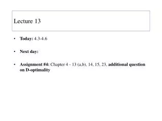
Lecture 13. Today we will Examine how the logic gate model (RC circuit) reacts to a sequence of input changes Relate these results to clocking speed Define propagation delay Introduce digital logic gates Examine how signals propagate through logic circuits. Vin. Vin. Vout. Vout. time.

E N D
Lecture 13 Today we will • Examine how the logic gate model (RC circuit) reacts to a sequence of input changes • Relate these results to clocking speed • Define propagation delay • Introduce digital logic gates • Examine how signals propagate through logic circuits
Vin Vin Vout Vout time time 0 0 Vin time 0 Sequential Switching • What if we step up the input to a logic circuit, • wait for the output to respond, • then bring the input back down to perform the next computation?
R + Vout(t) – Vin(t) + C Pulse width = RC Pulse width = 10RC 6 5 6 4 5 3 4 Vin, Vout Vin, Vout 2 3 1 2 0 1 0 1 2 3 4 5 0 Time 0 5 10 15 20 25 Time Pulse Distortion We need to wait for the output to reach a recognizable logic level, before changing the input again. This affects clock speed.
Example • Suppose that the capacitor is discharged at t=0. • With Vin(t) as shown, find Vout(t). 2.5 kW Vin(t) + Vout(t) – 4 V Vin(t) + 1 nF t 5 ms
Example • First, Vout(t) will approach 4 V exponentially. • We write the equation for this part using: • Initial condition Vout(0) = 0 V • Final value Vout,f= 4 V • Time constant RC = (2.5 kW)(1 nF) = 2.5 ms Vout(t) = Vout,f + (Vout(0)-Vout,f)e-t/RC Vout(t) = 4-4e-t/2.5ms V for 0 ≤ t ≤5 ms
Example • Then, at 5 ms, Vout(t) will approach 0 V exponentially. • We write the equation for this part using: • Initial condition Vout(5 ms) = ? Use equation from previous step, since Vout is continuous. Vout(5ms) = 4-4e-5ms/2.5ms= 3.44 V • Final value Vout,f= 0 V • Time constant RC = (2.5 kW)(1 nF) = 2.5 ms Vout(t) = Vout,f + (Vout(t0) -Vout,f)e-(t-t0)/RC Vout(t) = 3.44e-(t-5ms)/2.5ms for t > 5 ms
4 3.5 3 2.5 2 1.5 1 0.5 0 0 2 4 6 8 10 Example Vin(t) Vout(t) t (ms) { 4-4e-t/2.5ms for 0 ≤ t ≤5 ms 3.44e-(t-5ms)/2.5ms for t > 5 ms Vout(t) =
Design Issues • How long between successive inputs? • Need output to reach recognizable logic level • Output must be at this level long enough to serve as input to next logic gate • How many consecutive logic gates does signal go through before being “cleaned up” or saved in static memory cell? • Eventually the signal gets really bad • But adding hardware adds cost and delay
Propagation Delay • Suppose an input goes from some initial voltage to some final voltage. • In our examples, the input switch is immediate, but in practice it is not. • Propagation delay is officially defined as: (time when output is halfway to final value) minus (time when input is halfway to final value)
4 3.5 3 2.5 2 1.5 1 0.5 0 0 2 4 6 8 10 Illustration Using our equation for Vout(t), we can find: tP,LH (time when Vout(t) = 2 V, as it goes from 0 V to 4 V) – 0 s tP,HL (time when Vout(t) = 1.72 V, as it goes from 3.44 V to 0 V) – 5 ms tP,LH tP,HL tP,HL = tP,LH = 1.725 ms
Propagation Delay • It’s not a coincidence that the propagation delays were the same. • For a general RC circuit that has an input voltage switch at t = t0, Vout(t) = Vout,f + (Vout(t0) -Vout,f)e-(t-t0)/RC • The time when Vout(t) is ½ (Vout,f + Vout(t0))is given by ½ (Vout,f + Vout(t0)) = Vout,f + (Vout(t0) -Vout,f)e-(t-t0)/RC • Simplifying, ½ = e-(t-t0)/RC t = (ln 2)(RC) + t0 • The propagation delay, the difference between this time and t0, is tP = (ln 2)(RC) Depends only on time constant!
Graphing Propagation through Multiple Logic Gates • We will want to examine how these RC-related delays affect a signal going through multiple logic gates. • The math involved in putting an RC output (decaying exponential) into another RC circuit is not so easy. • So, when analyzing a circuit with many logic gates, we will use the following simplification: V V → → t tP Logic Gate t 0
Logic Gates • We have been using a simple RC circuit to model a logic gate. • In each case, the final value of Vout was Vin. • This will not always be true; sometimes, the output will go to logic 0 when the input is logic 1 and vice-versa. • To determine what the final value of a logic gate output will be, we need to learn the types of logic gates.
AND A C=A·B B A C=A+B OR B A B (EXCLUSIVE OR) Logic Gates A NAND C = B A NOR B NOT A XOR
Logic Functions: Truth Tables We specify what a logic circuit does by listing the output for each possible input. This listing is called a truth table. NOT AND NAND
Logic Functions: Truth Tables OR NOR XOR XNOR
Timing Diagrams • Now let’s look at how signals propagate through logic gates, taking delay into consideration. • Sketch the output for each logic gate in a more complicated circuit. A, B A A 1 (A)·B t B 0 Invalid info! A (A)·B 1 1 t t 0 tP 0 tP 2tP
Strategy for Timing Diagrams To find the output for a particular gate, • Graph the inputs for that gate • Graph the result of the logic gate using the input graphs • Shift right by one tP
Example A B D C A, B, C 1 t 0
Example A B D C B A+C 1 1 t t 0 tP 0 tP (B)·C D 1 1 t t 0 tP 2tP 2tP 3tP 0