Download
1 / 20
200 likes | 203 Views
This chapter explores different categories of I/O devices, including human interaction devices, machine-readable devices, and communication devices. It also discusses data rates for various I/O devices and different control methods. Operating system design issues, I/O buffering, and performance parameters for hard disk drives and solid-state drives are also covered.

E N D
I/O Management and Disk Scheduling Chapter 11
I/O Devices Categories: • For Human interaction: Printers, terminals, keyboard, mouse • Machine readable: Disks, Sensors, Controllers, Actuators … • Communication: Modems, Network cards, etc. • Differences: • Data rate: several orders of magnitude difference between transfer rates • Applications: e.g. Disk - store files, databases, virtual pages for MMU… • Complexity of control: e.g. Printer – simple control interface; disk – more complex • Unit of transfer: e.g. stream of bytes for a terminal or in blocks for a disk • Data representation: Different encoding schemes (e.g. parity conventions)
Data Rates for some I/O Devices HDMI v 2.0 (2.25 GB/s) 10 Gigabit Ethernet (1.25 GB/s) USB 3.0 (625 MB/s) SSD (500 MB/s) Firewire 3200 (393 MB/s) HardDisk HDD (140 MB/s) Gigabit Ethernet (125 MB/s) Firewire 800 (98 MB/s) USB 2.0 (1.5 MB/s) Modem (144 kB/s) Mouse serial port (150 B/s) 101 102 103 104 105 106 107 108 109 1010 Data Rate (Byte/s)
I/O Control Methods • Programmed I/O • one byte/word at a time • uses polling wastes CPU cycles • suitable for special-purpose micro-processor-controlled devices • Interrupt-driven I/O • many I/O devices use this approach as a good alternative to polling whenever it is needed • Direct Memory Access (DMA) • For block transfers • minimum CPU participation (only at the beginning and at the end)
Direct Memory Access • Takes control of the system from the CPU to transfer data to and from memory over the system bus • Only one bus master, usually the DMA controller due to tight timing constraints. • Cycle stealing is used to transfer data on the system bus. i.e. the instruction cycle is suspended so that data can be transferred by DMA controller in bursts. CPU can only access the bus between these bursts • No interrupts occur (except at the end)
Operating System Design Issues • Efficiency • Most I/O devices are extremely slow compared to main memory • I/O cannot keep up with processor speed • Use of multiprogramming allows for some processes to be waiting on I/O while another process executes • Swapping is used to bring in additional ready processes • Generality • Desirable to handle all I/O devices in a uniform manner • Hide the details of device I/O in lower-level routines. Processes and upper levels see devices in general terms such as read, write, open, close, lock, unlock
I/O Buffering • Reasons for buffering • If buffering is not used, the process which is waiting for I/O to complete can not be swapped out because the pages involved in the I/O must remain in RAM during I/O. • Overlap I/O with processing and increase efficiency • Block-oriented: Data is stored/transferred in fixed-size blocks (e.g. disks, tapes) • Stream-oriented: Data is transferred in streams of bytes (e.g. terminals, printers, communication ports, mouse, etc.)
Single Buffer • OS assigns a system buffer in main memory for an I/O request • Input transfers made to buffer • Block is moved to user space when needed. User process can process one block of data while another block is moved into the buffer • Swapping of user process is allowed since input is taking place in system memory, not user memory T =Disk I/O Time M = time to move the data into user space C = Computation Time No Buffer Time = T + C Single Buffer Time = Maximum[ C, T ] + M (overlap I/O with computation)
Double Buffer • A process can transfer data to or from one buffer while the OS empties or fills the other one T = Disk I/O Time C = Computation Time M = time to move the data into user space If (C + M) < T I/O device is working at full speed If (C + M) > T add more I/O buffers to increase efficiency! • Circular buffer used when more than two buffers are needed and the I/O operation must keep up with the process
HDD Performance Parameters • To read/write: disk head must be positioned at the right track and sector • Seek time: position the head at the desired track • Rotational delay (latency): time it takes for the beginning of the sector to reach the head Access time = seek time + rotational delay • Data transfer occurs as the sector moves under the head • HD Drive Parameters in 2010 • Seek times: 3-15ms, varies w distance (avg 8-10ms - improving at 7-10% per yr) • Rotation speeds: 5400 - 15,000 RPMs (avg. 2-5ms - improving at 7-10% per yr) • Data Transfer rates: 0.5 - 1.6 Gb/s
Solid State Drive (SSD) Also known as solid-state disk or electronic disk • SSDshave no moving mechanical components which distinguishes them from traditional HDDs • uses electronic interfaces compatible with traditional HDDs • More resistant to physical shock, run more quietly, have lower access time and less latency • But, SSDs are more expensive per unit of storage than HDDs. • While SSDs are more reliable than HDDs, SSD failures are often catastrophic, with total data loss. Whereas HDDs often give warning to allow much or all of their data to be recovered
Disk Scheduling Policies for HDDs • For a single disk there will be a number of I/O requests • If requests are serviced randomly worst possible performance • Access time is the reason for differences in performance Based on the Requester • First-in, First-out (FIFO) • Fair to all processes • Priority by Process (PRI) • Short batch jobs and interactive jobs may have higher priority • Good interactive response time • Last-in, First-out (LIFO) • Good for transaction processing systems • The device is given to the most recent user so there is little arm movement • Starvation is possible if a job is fallen back from the head of the queue
Disk Scheduling (cont.) Based on the Requested Item • Shortest Service Time First (SSTF) • Always choose the minimum Seek time and select the one that requires the leastmovementof the disk arm from its current position • SCAN (Elevator Algorithm) • Arm moves in one direction only, satisfying all outstanding requests until it reaches the last track in that direction. Then direction is reversed • C-SCAN (Circular SCAN) • Restricts scanning to one direction only (i.e. like a typewriter), After one scan, the arm is returned to the beginning to start a new scan. This reduces the maximum delay experienced by new requests. • N-step-SCAN • Segments the disk request queue into subqueues of length N which are processed one at a time, using SCAN • New requests added to other queues while the current queue is processed • FSCAN • two queues; one queue is serviced while the other is filled with new requests
RAID (Redundant Array of Independent Disks) • The rate of improvement in secondary storage performance has been much less than that of the microprocessor • Use many disks in parallel to increase storage bandwidth, also improve reliability • Files are striped across disks • Each stripe portion is read/written in parallel • Bandwidth increases with more disks • Redundancy is added to improve reliability RAID 0 disk array but No redundancy
RAID 1 (mirrored) • Redundancy is achieved by duplicating all the data • Each logical strip is mapped to two separate physical disks • A read request can be serviced by either of the two disks • A write request requires that both strips be updated; but can be done in parallel real-time back-up • When a drive fails, data can still be accessed from the mirror disk • Disadvantage: cost is doubled • typically limited to drives that store highly critical data and system software
RAID 2 (error detection/correction) • The strips are small; a single bit • an error-correcting code is calculated across corresponding bits on each data disk, and bits of the code are stored in the corresponding bit positions on multiple parity disks. • Typically Hamming code is used to be able to correct single-bit errors and detect double-bit errors. • Costly; only useful when disk errors are very high; since disks are pretty reliable not used in practice
RAID 3 (Bit-interleaved parity) • The strips are small; a single byte or a word • Single redundant disk • A simple parity bit is computed for the set of individual bits in the same position on all of the disks
Disk Cache • Buffer in main memory for disk sectors • Contains a copy of some of the sectors on the disk Least Recently Used (LRU) policy • The block that has been in the cache the longest with no reference to it is replaced IMPLEMENTATION • The cache consists of a stack of blocks • When a block is referenced, it is placed on the top of the stack • The block on the bottom of the stack is removed when a new block is brought in • Blocks don’t actually move around; pointers to the blocks are moved