Download
1 / 239
2.65k likes | 2.92k Views
Control Systems. Lecture 1 Introduction. Course information. Required Textbook: Modern Control Systems, Richard C. Dorf and Robert H. Bishop , Prentice Hall, 12th edition, 2010, ISBN-10: 0-13-602458-0. Math Prerequisites. Complex Numbers Add, Subtract, Multiply, Divide Linear Algebra

E N D
Control Systems Lecture 1 Introduction
Course information • Required Textbook: • Modern Control Systems, Richard C. Dorf and Robert H. Bishop, Prentice Hall, 12th edition, 2010, ISBN-10: 0-13-602458-0
Math Prerequisites • Complex Numbers • Add, Subtract, Multiply, Divide • Linear Algebra • Matrix Multiply, Inverse, Sets of Linear Eq. • Linear Ordinary Differential Equations • Laplace Transform to Solve ODE’s • Linearization • Logarithms • Modeling of Physical Systems • Mechanical, Electrical, Thermal, Fluid • Dynamic Responses • 1st and 2nd Order Systems of ODE’s
Prerequisites: Complex Numbers • Ordered pair of two real numbers • Conjugate • Addition • Multiplication
Complex Numbers • Euler’s identity • Polar form • Magnitude • Phase
Logarithm • The logarithm of x to the base b is written • The logarithm of 1000 to the base 10 is 3, i.e., • Properties: Why?
Summary & Exercises • Prerequisites • Complex numbers, Linear Algebra, Logarithm, Laplace transform • Dynamics • Next • Introduction • Exercises • Buy the course textbook and keep it! • Review today’s slides on complex numbers and logarithm • Read Chapter 1 and 2 of the textbook.
What is “Control”? • Make some object (called system, or plant) behave as we desire. • Imagine “control” around you! • Room temperature control • Car/bicycle driving • Voice volume control • “Control” (move) the position of the pointer • Cruise control or speed control • Process control • etc.
What is “Control Systems”? • Why do we need control systems? • Convenient (room temperature control, laundry machine) • Dangerous (hot/cold places, space, bomb removal) • Impossible for human (nanometer scale precision positioning, work inside the small space that human cannot enter) • It exists in nature. (human body temperature control) • Lower cost, high efficiency, etc. • Many examples of control systems around us
Open-Loop Control • Open-loop Control System • Toaster, microwave oven, shooting a basketball • Calibration is the key! • Can be sensitive to disturbances input output Signal Input Controller (Actuator) Plant
Example: Toaster • A toaster toasts bread, by setting timer. • Objective: make bread golden browned and crisp. • A toaster does not measure the color of bread during the toasting process. • For a fixed setting, in winter, the toast can be white and in summer, the toast can be black (Calibration!) • A toaster would be more expensive with sensors to measure the color and actuators to adjust the timer based on the measured color. Setting of timer Toasted bread Toaster
Example: Laundry machine • A laundry machine washes clothes, by setting a program. • A laundry machine does not measure how clean the clothes become. • Control without measuring devices (sensors) are called open-loop control. Program setting Washed clothes Machine
Closed-Loop (Feedback) Control • Compare actual behavior with desired behavior • Make corrections based on the error • The sensor and the actuator are key elements of a feedback loop • Design control algorithm Signal Input Error output Plant Actuator Controller + - Sensor
Ex: Automobile direction control • Attempts to change the direction of the automobile. • Manual closed-loop (feedback) control. • Although the controlled system is “Automobile”, the input and the output of the system can be different, depending on control objectives! Steering wheel angle Desired direction Error Direction Auto Brain Hand Eye
Ex: Automobile cruise control • Attempts to maintain the speed of the automobile. • Cruise control can be both manual and automatic. • Note the similarity of the diagram above to the diagram in the previous slide! Disturbance Error Desired speed Acceleration Speed Auto Controller Actuator Sensor
Basic elements in feedback control systems Disturbance Error Reference Output Input Controller Actuator Plant Sensor Control system design objective To design a controller s.t. the output follows the reference in a “satisfactory” manner even in the face of disturbances.
Systematic controller design process Disturbance Reference Output Input Controller Actuator Plant Sensor 4. Implemenation 1. Modeling Controller Mathematical model 2. Analysis 3. Design
Goals of this course To learn basics of feedback control systems • Modeling as a transfer function and a block diagram • Laplace transform (Mathematics!) • Mechanical, electrical, electromechanical systems • Analysis • Step response, frequency response • Stability: Routh-Hurwitz criterion, (Nyquist criterion) • Design • Root locus technique, frequency response technique, PID control, lead/lag compensator • Theory, (simulation with Matlab), practice in laboratories
Course roadmap Modeling Analysis Design • Laplace transform • Transfer function • Models for systems • mechanical • electrical • electromechanical • Linearization • Time response • Transient • Steady state • Frequency response • Bode plot • Stability • Routh-Hurwitz • (Nyquist) Design specs Root locus Frequency domain PID & Lead-lag Design examples (Matlab simulations &) laboratories
Goals of this course To learn basics of feedback control systems • Modeling as a transfer function and a block diagram • Laplace transform (Mathematics!) • Mechanical, electrical, electromechanical systems • Analysis • Step response, frequency response • Stability: Routh-Hurwitz criterion, (Nyquist criterion) • Design • Root locus technique, frequency response technique, PID control, lead/lag compensator • Theory, (simulation with Matlab), practice in laboratories
Laplace transform • One of most important math tools in the course! • Definition: For a function f(t) (f(t)=0 for t<0), • We denote Laplace transform of f(t) by F(s). (s: complex variable) f(t) F(s) t 0
Examples of Laplace transform f(t) • Unit step function • Unit ramp function 1 t 0 (Memorize this!) f(t) t 0 (Integration by parts)
EX. Integration by parts
Examples of Laplace transform (cont’d) f(t) Width = 0 Height = inf Area = 1 • Unit impulse function • Exponential function t 0 (Memorize this!) f(t) 1 t 0
Examples of Laplace transform (cont’d) • Sine function • Cosine function (Memorize these!) Remark: Instead of computing Laplace transform for each function, and/or memorizing complicated Laplace transform, use the Laplace transform table !
Laplace transform table Inverse Laplace Transform
Properties of Laplace transform1.Linearity Ex. Proof.
Properties of Laplace transform2.Time delay Ex. f(t) f(t-T) Proof. 0 T t-domain s-domain
Properties of Laplace transform3.Differentiation Ex. Proof. t-domain s-domain
Properties of Laplace transform4.Integration Proof. t-domain s-domain
Properties of Laplace transform5.Final value theorem Ex. if all the poles of sF(s) are in the left half plane (LHP) Poles of sF(s) are in LHP, so final value thm applies. Ex. Some poles of sF(s) are not in LHP, so final value thm does NOT apply.
Properties of Laplace transform6.Initial value theorem Ex. if the limits exist. Remark: In this theorem, it does not matter if pole location is in LHS or not. Ex.
Properties of Laplace transform7.Convolution Convolution IMPORTANT REMARK
Summary & Exercises • Laplace transform (Important math tool!) • Definition • Laplace transform table • Properties of Laplace transform • Next • Solution to ODEs via Laplace transform • Exercises • Read Chapters 1 and 2. • Solve Quiz Problems.
ME451: Control Systems Lecture 3 Solution to ODEs via Laplace transform
Course roadmap Modeling Analysis Design • Laplace transform • Transfer function • Models for systems • electrical • mechanical • electromechanical • Block diagrams • Linearization • Time response • Transient • Steady state • Frequency response • Bode plot • Stability • Routh-Hurwitz • Nyquist Design specs Root locus Frequency domain PID & Lead-lag Design examples (Matlab simulations &) laboratories
Laplace transform (review) • One of most important math tools in the course! • Definition: For a function f(t) (f(t)=0 for t<0), • We denote Laplace transform of f(t) by F(s). (s: complex variable) f(t) F(s) t 0
An advantage of Laplace transform • We can transform an ordinary differential equation (ODE) into an algebraic equation (AE). t-domain s-domain AE ODE 1 2 Partial fraction expansion Solution to ODE 3
Example 1 ODE with initial conditions (ICs) • Laplace transform
Properties of Laplace transformDifferentiation (review) t-domain s-domain
Example 1 (cont’d) unknowns • Partial fraction expansion Multiply both sides by s & let s go to zero: Similarly,
Example 1 (cont’d) • Inverse Laplace transform If we are interested in only the final value of y(t), apply Final Value Theorem:
Example 2 • S1 • S2 • S3
In this way, we can find a rather complicated solution to ODEs easily by using Laplace transform table!
Example: Newton’s law We want to know the trajectory of x(t). By Laplace transform, M (Total response) = (Forced response) + (Initial condition response)
EX. Air bag and accelerometer • Tiny MEMS accelerometer • Microelectromechanical systems (MEMS) (Pictures from various websites)
Ex: Mechanical accelerometer (cont’d) • We would like to know how y(t) moveswhen unit step f(t) is applied with zero ICs. • By Newton’s law
Ex: Mechanical accelerometer (cont’d) • Suppose that b/M=3, k/M=2 and Ms=1. • Partial fraction expansion • Inverse Laplace transform
Summary & Exercises • Solution procedure to ODEs • Laplace transform • Partial fraction expansion • Inverse Laplace transform • Next, modeling of physical systems using Laplace transform • Exercises • Derive the solution to the accelerometer problem. • E2.4 of the textbook in page 135.