Download
1 / 25
260 likes | 428 Views
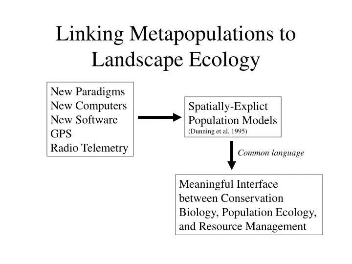
Linking Metapopulations to Landscape Ecology. New Paradigms New Computers New Software GPS Radio Telemetry. Spatially-Explict Population Models (Dunning et al. 1995). Common language. Meaningful Interface between Conservation Biology, Population Ecology, and Resource Management. Topics.

E N D
Linking Metapopulations to Landscape Ecology New Paradigms New Computers New Software GPS Radio Telemetry Spatially-Explict Population Models (Dunning et al. 1995) Common language Meaningful Interface between Conservation Biology, Population Ecology, and Resource Management
Topics • Basics of Modeling • Sensitivity Analysis • Use in Wildlife Management • Predicting response to habitat change • Determining harvest • Anticipating exotic species spread • Conserving and reintroducing endangered species • Assessing risk
SEPMs • Goal: Model population dynamics in realistic setting so that effects of various land management options or global change scenarios on wildlife populations can be appraised • Data Intensive: Habitat-specific demography, dispersal, habitat selection
Two Approaches • Each cell contains an individual (cell size = territory or home range size) • Equations to describe daily decisions to forage, avoid predators, etc that eventually is translated to individual growth • Equations to describe yearly decisions to breed or disperse and tie this to survival and reproductive output, then to lambda at annual time intervals • Each cell contains a population (cell size is a deme) • Equations to model birth, death, immigration, emigration
Sensitivity Analysis • Often most important output of model when knowledge is less than perfect • Determine relative importance of model parameters to population change • Focus future research • Identify processes of management concern • Bachman’s Sparrows (Pulliam et al. 1992) • Adult Survival Sx = 1.4 • Juvenile Survival Sx = 1.2 • Mature Habitat Sx = 0.92 • Reproduction Sx = 0.51 • Dispersal Mortality Sx = 0.04
Timber Harvest and Bachman’s Sparrow (Liu et al. 1995) Non-target management species (target was RCWP)
Simulating Effects of Various Harvest Scenarios Through Time Sparrows will return to acceptable level after going through a bottleneck, but return time depends on timber harvest scenario—random harvest is poorest scenario
Historic Change In Moose Density (McKenney et al. 1998) Identifying where populations have increased or decreased through time helps managers decide where to harvest in future
Predicting Change in Spread of Exotic Species (Rushton et al. 1997) Gray Squirrel (Pest in UK) Red Squirrel (Native in UK)
Determining Habitat Needs of an Endangered Species (Letcher et al. 1998) Model of extremely complex sociality of Red-cockaded Woodpeckers
Sensitivity Analysis Fledgling Production Female Breeder Mortality Female Disperser Mortality have strong effects on population growth
Spatial Arrangement of Habitat is Likely Important Population growth depends on number of territories (amount of habitat) and how they are arranged (clumping of habitat)
Research at Larger Scale Shows Importance of Dispersal Habitat to Bighorn Management Extinct Extant • Intermountain travel corridors needed • Domestic sheep free to decrease disease spread • Focus traditionally at the local scale • need to switch to metapopulation scale • Sheep in Santa Catalina Mountains (Arizona) are likely to be next to go extinct • management of herd and local habitat not enough • settlement, roads, agriculture have made intermountain travel nearly impossible (Krausman 1997)
Ecological Niche Models • Model species’ ecological niches and predict geographic distribution (Martinez-Meyer et al. 2006) • Ecological conditions that can maintain populations without immigration • Model the conditions where species occurs and use these to predict where similar conditions are met elsewhere • Assess how these conditions change with extrinsic factors like climate, landcover conversion, etc. Fig. 1 Known occurrence points (circles) of California condor in southern California, and results of GARP analysis predicting the potential geographic distribution south to northern Baja California. Confidence in prediction of potential presence is shown as a greyscale gradient from white (no confidence) to black (high confidence). Inset shows final areas (dark polygons) selected as optimal for reintroductions: areas predicted habitable at present and not in the future are shown in light grey; areas predicted habitable at present and in the future are in black; areas predicted not habitable at present but that are predicted to become habitable in the future are in dark grey.
Example of finding Reintroduction Sites for Wolves and Condors Fig. 2 Process of identifying suitable areas for reintroductions of California condors in Mexico: (A) raw GARP prediction that reflects overall suitability of climates and landscapes, (B) cutting by distribution of primary vegetation in the region, (C) weighting by distance to human presence (roads and settlements), and (D) weighting by future climate suitability. Confidence in prediction of potential presence is shown as a greyscale gradient from white (no confidence) to black (high confidence).
Choice and Risk Models of Habitat Quality • Nielsen et al. article on grizzly conservation in Alberta (required read and for discussion) • Risk to nesting marbled murrelets
Days to predation for all eggs (depredated and non-depredated eggs)(the darker the color the lower the predation) Days to pred = 8.04 – 8.16 landscape patch density at 5km + 1.10 landscape contrast weighted edge density at 2km – 10.31 Shannon-Weaver evenness index at 2km (r2 = 0.27)
Stands used to test model (2000 and 2001) • Test of models observed vs. predicted: • Percent eggs: r= 0.22, p=0.19 • Percent eggs and chicks depredated: not tested because only eggs used to test model • Days to predation: r=0.29, p=0.07
Applicability of model: Songbird study sites (green low, blue high predation) • Low n = 8 • High n = 9
Species Studied • Sub-Canopy: • Pacific-slope Flycatcher • American Robin • Shrub: • Swainson’s Thrush • Ground: • Wilson’s Warbler • Song Sparrow • Dark-eyed Junco • Winter Wren
Surveys • Point count predators (Luginbuhl et al. 2001) • Point counts for songbirds • Map location of all detections every 2 weeks • Spot map songbird breeding behavior (Vickery Index of Success: cumulative over season; rank 1 – 7) • Find and monitor nests (Mayfield mortality rates)
Predators more numerous in high predation areas (n = 8) p = 0.07
Nesting success differs for the American robin and subcanopy nesters p = 0.003 p = 0.01 11 58 31 10 16 4 33 17 12 4 6 4
Discussion • In small groups consider the Nielsen et al. paper • How did they model habitat quality? • How does habitat quality influence their proposed conservation strategy? • Is the conservation strategy realistic to apply in Alberta? • What would you do next to improve grizzly models?
References • Rushton, SP, Lurz, PWW, Fuller, R., and PJ Garson. 1997. Modelling the distribution of the red and grey squirrel at the landscape scale: a combined GIS and population dynamics approach. J. Animal Ecology 34:1137-1154. • Liu, J., JB Dunning, Jr., and HR Pulliam. 1995. Potential effects of a forest management plan on Bachman’s Sparrows (Aimophila aestivalis): Linking a spatially explicit model with GIS. Conservation Biology 9:62-75. • Pulliam, HR, JB Dunning, Jr., and J. Liu. 1992. Population dynamics in complex landscapes: a case study. Ecological Applications 2:165-177. • Dunning, JB, Jr., DJ Stewart, BJ Danielson, BR Noon, TL Root, RH Lamberson, and EE Stevens. 1995. Spatially explicit population models: current forms and future uses. Ecological Applications 5:3-11. • McKenney, DW, Rempel, TRS, Venier, LA, Wang, Y, and AR Bisset. 1998. Development and application of a spatially explicit moose population model. Canadian Journal of Zoology 76:1922-1931. • Martinez-Meyer, E., Peterson, A. T., Servin, J. I., and L. F. Kiff. 2006. Ecological niche modelling and prioritizing areas for species reintroductions. Oryx 40:411-418.