Download
1 / 26
270 likes | 477 Views
Risk Assessment . Vicki M. Bier (University of Wisconsin-Madison). Introduction. Risk assessment is a means to characterize and reduce uncertainty to support our ability to deal with catastrophe Modern risk assessment for engineered systems began with the Reactor Safety Study (1975):

E N D
Risk Assessment Vicki M. Bier (University of Wisconsin-Madison)
Introduction • Risk assessment is a means to characterize and reduce uncertainty to support our ability to deal with catastrophe • Modern risk assessment for engineered systems began with the Reactor Safety Study (1975): • Applications to engineered systems and infrastructure are common
What is Risk Assessment? • “A systematic approach to organizing and analyzing scientific knowledge and information for potentially hazardous activities or for substances that might pose risks under specified circumstances” • National Research Council (NRC), 1994
Definitions of Risk • “Both uncertainty and some kind of loss or damage” (Kaplan and Garrick 1981) • “The potential for realization of unwanted, negative consequences of an event” (Rowe 1976) • “The probability per unit time of the occurrence of a unit cost burden” (Sage and White 1980) • “The likelihood that a vulnerability will be exploited” (NRC 2002)
Paradigm for Risk Assessment • A form of systems analysis • Answers three questions (Kaplan and Garrick 1981): • “What can go wrong?” • “How likely is it that that will happen?” • “If it does happen, what are the consequences?”
What is Probabilistic Risk Assessment? • An integrated model of the response of an engineered system to disturbances during operations • A rigorous and systematic identification of the levels of damage that could conceivably result from those responses • A probabilistic (that is, quantitative) assessment of the frequency of such occurrences and our uncertainty in that assessment • A tool to help owners/operators make good decisions about system operations
ESSENCE OF PRA • A PRA is an assessment of how well a system responds to a variety of situations • It answers three basic questions:1. What can go wrong during operation?2. How likely is it to go wrong?3. What are the consequences when it goes wrong? • We answer the first question in terms of scenarios • We answer the second by quantifying our knowledge of the likelihood of each scenario • We answer the third by quantifying our knowledge of the response of the system and its operators in terms of:- damage states- release states and source terms- scenario consequences
GRAPHICAL PRESENTATION OF RISK P RISK CURVE p(>x) X
STRUCTURE OF THE MODERN PRA MODEL LEVEL 3 2 1 OFFSITE RADIOACTIVE MATERIAL DISPERSION AND HEALTH IMPACT MODEL CONTAINMENT STRENGTH AND CORE DAMAGE PROGRESSION MODEL RISK BY HEALTH EFFECT TYPE INITIATINGEVENTS PLANT (ACTIVE SYSTEMS) MODEL PLANTDAMAGE STATES RELEASE CATEGORIES FRONTLINE SYSTEMS – LATE AND CONTAINMENT SAFETY FEATURES RESPONSE MODEL FRONTLINE SYSTEMS – EARLY RESPONSE MODEL SUPPORT SYSTEMS MODEL SUPPORTSYSTEMSTATES SUBTREEFREQUENCIES
QUANTIFYING SCENARIOS INITIATINGEVENT x A B C D NODE B1 NODE A NODE C3
EVENT SEQUENCE QUANTIFICATION WHERE = the frequency of scenario S = the frequency of initiating event I = the fraction of times system Asucceeds given that I has happened = the fraction of times system Bfails given that I has happenedand A has succeeded = the fraction of times C succeedsgiven that I has happened, thatA has succeeded, and B has failed = the fraction of times D fails given INITIATINGEVENT A B C D 1 NODE B1 SIMPLIFIED EVENT TREE DIAGRAM
TANK STAGES TO EVENT TREE LINKING LATEFRONTLINESYSTEMS PLANTDAMAGESTATES EARLYFRONTLINESYSTEMS OTHERSUPPORTSYSTEMS ELECTRICPOWERSYSTEMS INITATINGEVENTS AFW SCOPINGREQUIREMENTS PUMP1 PUMP2 PUMP3
RELATIONSHIP OF FAULT TREES TO EVENT TREES INITIALCONDITIONS STAGE A TOP EVENTS DAMAGE STATE OK PLS LOC/V AFW PLS LOC/V LEGEND = “OR” GATE APUMODULE TANK = “AND” GATE ISOLATIONVALVE 1 ISOLATIONVALVE 2 GGVM COOLING 1 GGVM COOLING 2
FAULT TREES AND EVENT TREES • Both useful • Event trees used to display order of events and dependent events • Fault trees used to display combinations of events: • Order and dependencies are obscured • Logically equivalent
RISK MANAGEMENT • Develop an integrated plant-specific risk model • Rank order contributors to risk by damage index • Decompose contributors into specific elements • Identify options, such as design and procedure changes, for reducing the impact of the contributor on risk • Make the appropriate changes in the risk model: • And re-compute the risk for each option • Compute the cost impacts of each system configuration, relative to the base case: • Including both initial and annual costs • Present the costs, risks, and benefits for each option
RISK DECOMPOSITION(ANATOMY OF RISK) LEVEL OF DMAGE TYPE OF RELEASE TYPE OF PLANT DAMAGE INITIATING EVENT EVENT SEQUENCE SYSTEM UNAVAILABILITY FAILURE CAUSES System B Cause Table INPUT DATA • Initiating events • Components • Maintenance • Human error • Common cause • Environmental • Other CAUSES FREQUENCIES EFFECTS MAJOR SYSTEM DOMINANTSEQUENCE DOMINANT FAILURE MODES
REACTOR TRIP SYSTEM CAUSE TABLECONTRIBUTORS TO SYSTEM FAILURE FREQUENCY This analysis was performed in November 1982
Data Analysis • Input parameters are quantified from available data: • Typically using expert judgment and Bayesian statistics • Due to sparseness of directly relevant data • Hierarchical (“two-stage”) Bayesian methods common: • Partially relevant data used to help construct prior distributions • Numerous areas in which improvements can be made: • Treatment of probabilistic dependence • Reliance on subjective prior distributions • Treatment of model uncertainty
Dependencies • The failure rates (or probabilities) of components can be uncertain and dependent on each other: • For example, learning that one component had a higher failure rate than expected may cause one to increase one’s estimates of the failure rates of other similar components • Failure to take such dependence into account can result in substantial underestimation of the uncertainty about the overall system failure rate: • And also the mean failure probability of the system • Historically, dependencies among random variables have often been either ignored: • Or else modeled as perfect correlation
Dependencies • The use of copulas or other multivariate distributions has become more common: • But tractable models still are not sufficiently general to account for all realistic assumptions, such as E(X|D) > E(Y|D) for all D • High-dimensional joint distributions are also challenging: • Correlation matrices must be positive definite • There can be numerous higher-order correlations to assess • Cooke et al. developed a practical method for specifying a joint distribution over n continuous random variables: • Using only n(n1)2 assessments of conditional correlations • (Bedford and Cooke 2001; Kurowicka and Cooke 2004)
Subjectivity • PRA practitioners sometimes treat the subjectivity of prior distributions cavalierly: • Best practice for eliciting subjective priors is difficult and costly to apply • Especially for dozens of uncertain quantities • The use of “robust” or “reference” priors may minimize the reliance on judgment: • Although this may not work with sparse data
Probability Bounds Analysis • Specify bounds on the cumulative distribution functions of the inputs: • Rather than specific cumulative distributions • (Ferson and Donald 1998) • These bounds can then be propagated through a model: • The uncertainty propagation process can be quite efficient • Yielding valid bounds on the cumulative distribution function for the final result of the model (e.g., risk) • Can take into account not only uncertainty about the probability distributions of the model inputs: • But also uncertainty about their correlations and dependence structure • This is especially valuable: • Correlations are more difficult to assess than marginal distributions • Correlations of 1 or -1 may not yield the most extreme distributions for the output variable of interest (Ferson and Hajagos 2006)
Exposure to Contamination • Regan et al. (2002) compare a two-dimensional Monte Carlo analysis of this problem to the results obtained using probability bounds • The qualitative conclusions of the analysis (e.g., that a predator species was “potentially at risk” from exposure to contamination) remained unchanged: • Even using bounds of zero and one for some variables • Bounding analysis can help support a particular decision: • If results and recommendations are not sensitive to the specific choices of probability distributions used in a simulation
Model Uncertainty • Uncertainty about model form can be important • Assessing a probability distribution over multiple plausible models is frequently not reasonable: • “All models are wrong, some models are useful” (Box) • Models are not a collectively exhaustive set • Some models are intentionally simple or conservative • Bayesian model averaging avoids giving too much weight to complex models (Raftery and Zheng 2003): • But still relies on assigning probabilities to particular models • Using Bayes theorem to update those probabilities given data
Joint Updating • In general, one will be uncertain about both model inputs and outputs • One would like to update priors for both inputs and outputs consistently: • With the wider distribution being more sensitive to model results • Raftery et al. (1995) attempted this (Bayesian synthesis): • But that approach is subject to Borel’s paradox • Since it can involve conditioning on a set of measure zero • Joint updating of model inputs and outputs is largely an unsolved problem