Download
1 / 31
310 likes | 516 Views
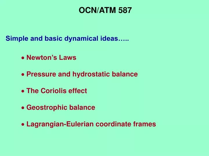
OCN/ATM 587. Simple and basic dynamical ideas…. Newton’s Laws Pressure and hydrostatic balance The Coriolis effect Geostrophic balance Lagrangian-Eulerian coordinate frames. Newton’s Laws…. [a 2nd order vector ODE or PDE; actually 3 scalar ODE/PDEs ]. where. the 3 ODEs are:.

E N D
OCN/ATM 587 Simple and basic dynamical ideas….. Newton’s Laws Pressure and hydrostatic balance The Coriolis effect Geostrophic balance Lagrangian-Eulerian coordinate frames
Newton’s Laws…. [a 2nd order vector ODE or PDE; actually 3 scalar ODE/PDEs ] where the 3 ODEs are: note notation variants:
Properties of an atmosphere and ocean at rest: Note that gases and liquids are fluids. Fluids differ from solids in that fluids at rest cannot support a shearing stress….the distinctive property of fluids. A fluid at rest cannot sustain a tangential force…the fluid would simply glide over itself in layers in such a case. At rest, fluids can only sustain forces normal to their shape (a container, for example). Pressure is the magnitude of such a normal force, normalized by the area of the fluid normal to the force. pressure = normal force / unit area [pressure is a scalar]
The pressure cube… Let Fp be the vector force per unit volume, in order to take the size of the cube out of the problem: Note:
The force/cube equations for all of the faces of the cube can be combined to yield the vector equation Suppose the force is redefined on a per unit mass basis; then This equation says, simply, that the net pressure force acting on a fluid element is given by the pressure gradient.
Pressure, continued….. If only pressure forces are acting on an element of fluid (air or seawater), then due to Newton’s Laws the element must be accelerating. If the pressure forces are balanced by some other force, then the fluid element can be in equilibrium (ie, at rest). What other forces are there? Consider gravity…
If the pressure force is balanced by the force of gravity, then or, [horizontal equations] [vertical equation] thehydrostatic relation
The hydrostatic relation…. which can be easily integrated. Oceanic case: assuming = constant If we define the pressure at the sea surface to be zero, then pressure at any depth can be calculated Note: SI units of pressure are pascals, but oceanographers typically use decibars; numerically the depth in meters is the same as the pressure in decibars.
Check the units (oceanic case)…. weight per unit area Notes… Depth (z) is negative – downwards. The hydrostatic pressure is just the weight of the water column above (per unit area).
Atmospheric case: p = RT [ideal gas law] For an isothermal atmosphere (T constant) the hydrostatic relation can be integrated to find that p = ps e-z/HH = RT/g [the scale height] Here psis the sea level pressure and H 7.6 km. Pressure decreases exponentially with altitude.
Variation of pressure with altitude in the atmosphere…. 90 Eq ps 1000 mbar
When can the hydrostatic relation be used? (ie, what has been assumed here?) We assumed that pressure forces balance gravity…..when will this be true? But suppose instead that
As long as the flow will still be hydrostatic. for L = 1 meter, this will be true as long as T 1 sec (ocean) for L = 1 km, this will be true as long as T 30 sec (atmosphere)
pressure (continued)…… p high p low p p Fm [thus, a force equal to Fm is needed to balance the pressure force]
The Coriolis effect…. (i) Motion on a nonrotating Earth The motion is determined by Newton’s Laws with gravity, Example: projectile motion Note: Newton’s Laws as normally used are true only in an inertial coordinate frame (one fixed with respect to distant, fixed stars. An Earth-based coordinate system (longitude, latitude, altitude; east, north, up) is not an inertial coordinate system.
Coriolis effect, continued • (ii) Stationary motion on a rotating Earth • The motion is determined by Newton’s Laws with gravity; the motion is only stationary in an Earth-based coordinate system [ east, north, up; longitude, latitude, altitude]. Motion in an Earth-based coordinate system leads to a new effect: the centrifugal force. [inertial frame: centripetal acceleration] [rotating frame: centrifugal force]
Coriolis effects….continued On a rotating Earth the effective gravity is the sum of the force of attraction and the centrifugal force.
Coriolis effect, continued (iii) Moving particles on a rotating Earth The motion is determined by Newton’s Laws with gravity; the motion is not stationary in an inertial frame or the rotating frame. Motion in the rotating frame leads to a new effect: the Coriolis force.
Coriolis effect (continued)…. • Moving a distance L between A and B at speed Uo requires a time L/Uo . • Earth rotation rate = • Earth rotation time= 1/ • = (Earth time)/(AB time) = Uo/(L) • << 1 (slow AB motion, strong rotation) • >> 1 (fast AB motion, weak rotation) A point on latitude is rotating at a tangential velocity VT given by VT = V0 cos , where V0 is the equatorial value.
Coriolis effect (continued)…. i, j, k = east, north, up unit vectors Coriolis acceleration = 2 u u = (u, v, w) Coriolis force = 2 u
Coriolis effect, continued…. Initial velocity Coriolis force north (0,v,0), v>0 east south (0,v,0), v<0 west east (u,0,0), u>0 south, up west (u,0,0), u<0 north, down up (0,0,w), w>0 west down (0,0,w), w<0 east The Coriolis effect is due to rotation + spherical geometry
Coriolis effect (continued)…. Newton’s Laws with rotation: or
Coriolis effect, continued…. add the pressure gradient as a force steady or nearly steady motion geostrophic balance geostrophic flow: pressure gradient balances the Coriolis force flow is along lines of constant pressure
The Coriolis effect and geostrophic balance…. Recall the equation for the Coriolis acceleration: Note in the i term that (w cos )/(v sin) = (w/v) cot << 1, except near the Equator. So, neglect the w term with respect to the v term. Also, note that we have already examined hydrostatic balance and found that vertical accelerations are small compared to horizontal. Thus, ignore the k term here.
Coriolis effect and geostrophic motion…. With these simplifications the geostrophic equations become +x pressure gradient:northward flow in the N. hemisphere +y pressure gradient: westward flow in the N. hemisphere These equations provide a simple diagnostic tool for examining the circulation of the atmosphere or the ocean.
Coriolis effect (continued)…. H H L H L Weather map shows geostrophic flow
Lagrangian and Eulerian descriptions of motion…. Newton’s Laws are formulated in terms of the motion of a particle in an inertial reference frame. The Coriolis effect provides a modification to Newton’s Laws for a rotating frame. What happens if we don’t want to follow a particle, but instead prefer to examine the flow on a grid? This is the type of observation made by ships on a regular survey pattern or at fixed weather stations. This situation is not included in Newton’s Laws, but we can easily modify the Laws to allow this description. Lagrangian description: following a particle Eulerian description: on a grid (fixed points)
Eulerian and Lagrangian descriptions…. Consider some property that we want to measure, where = (x, y, z, t), and (x0, y0, z0) is a fixed point. In the vicinity of (x0, y0, z0) , we can write that
Lagrangian-Eulerian descriptions…. This can be rearranged to yield Taking the limit as the terms go to zero, it is found that Lagrangian Eulerian (total) (local) (motion)
Newton’s Laws…. The Eulerian version of Newton’s Laws with rotation are [note: this vector equation has no general solution]