Download
1 / 30
300 likes | 400 Views
Earth. http://weather.uwyo.edu/surface/front.html. Last time - introduced : Mass density ρ = Mass/Volume Number density n = No. of molecules/Volume and therefore, ρ = n x m where m is the mass of each molecule. In general, m = M/N A

E N D
Last time - introduced: Mass density ρ = Mass/Volume Number density n = No. of molecules/Volume and therefore, ρ = n x m where m is the mass of each molecule. In general, m = M/NA where M is the gram molecular weight of the gas and NA is Avogadro’s number.
Mass density, ρ ρ = number x molecular per volume mass ρ = n x m Near sea level, nair = 2.72 x 1019 cm-3 (T = 273 °K or 0 ºC) and mair = 4.81 x 10⁻²³ gm so ρair = 1.3 x 10⁻³ gm/cm3 or ρair = 1.3 kg/m3 NOTE: ρairdepends on pressure (or altitude) and the air temperature.
Gas Law p = n k T where n = number density (or number/volume) and k = Boltzmann’s constant = 1.38 x 10⁻¹⁶°K (cgs units) = 1.38 x 10⁻²³°K (mks units) and the temperature, T, is in degrees Kelvin Basically, p = (Number/Volume) x Temperature or p x V = (Constant) x T
In cgs units, at sea level Pressure = Mass/Area x g = 1033 gm/cm2 x 980.6 cm/sec2 = 1.013 x 10⁶ dynes/cm2 = 1.013 bars (b) = 1013 mb where 1 bar = 106 dynes/cm2 and 1 mb = 103 dynes/cm2
In mks units, at sea level patm = 1.013 x 10⁵ Pascals (Pa) = 101.3 kiloPascals (kPa) = 1013 hectoPascals (hPa) Note: 1 mb = 100 Pa = 1 hPa (hectoPascal)
What is the number density of normal air at sea level? From the gas law, p = n k T We can say that n = p/kT so plugging in k = 1.38 x 10⁻¹⁶ cgs units T = 298 °K (75 °F) p = 1.013 x 10⁶ dynes/cm2 we get n = 2.5 x 1019 cm-3 Now, if we multiply by the average mass of an air molecule, we can obtain the mass density of air ρ = n m = 2.5 x 1019 cm-3 x 4.8 x 10-23 gm = 1.2 x 10⁻³ gm/cm3
Air pressure decreases rapidly (exponentially) with altitude.
“Surface” pressure that is measured is often not at sea level. Therefore, must add some pressure to correct for altitude of the weather station. Typically, add 1 mb for every 10 m of altitude. Example: In Tucson, altitude 730 m (2400 feet), measure about 930 mb; therefore, must add 73 mb to pressure to “reduce” the pressure to sea level or 930 mb + 73 mb = 1003 mb to correct for the altitude of the measuring station.
Average Sea Level Pressure June July August December January February
Good web address for upper air data is: http://weather.uwyo.edu/upperair/sounding.html
One way of visualizing jet streams is to consider a river. The flow in the river is usually strongest in the center and decreases as one approaches the river bank. It can be said that jetstreams are "rivers of air".
The wind blows from west to east in jet streams but the flow often shifts to the north and south.
Air – mixture of gases plus an aerosol Nitrogen (N2) 78.08 % Oxygen (O2) 20.95 Argon (Ar) 0.93 Water vapor (H2O) 1 to 4 Carbon dioxide (CO2) 0.038
Photosynthesis – source of oxygen Chlorophyll in plants acts as catalyst for production of carbohydrates 6CO2 + 6H2O + light C6H12O6 + 6O2
The distribution of water vapor in the atmosphere varies strongly with time, location and height, which makes it difficult to model. This image shows the distribution of water vapor in the Earth's atmosphere using model data from September 1996. The humid tropics (red) contain almost 100 times more water vapor than the dry poles (blue). [Physics World, May 1, 2003]