Download
1 / 50
500 likes | 507 Views
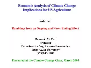
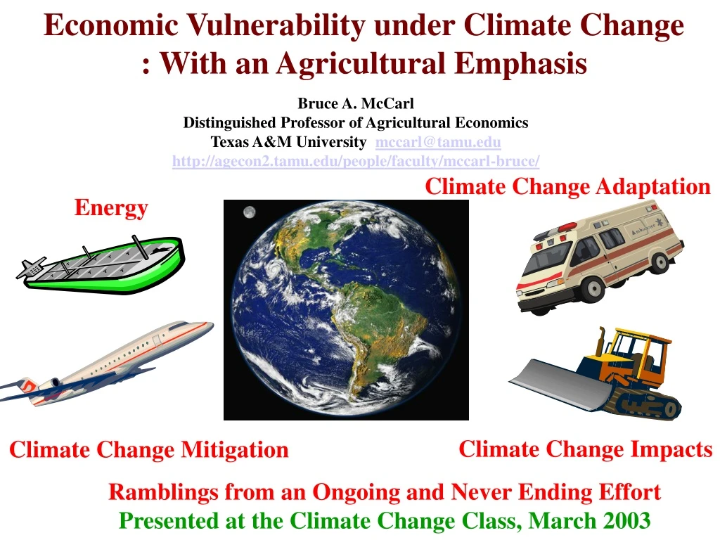
Economic Vulnerability under Climate Change : With an Agricultural Emphasis. Bruce A. McCarl Distinguished Professor of Agricultural Economics Texas A&M University mccarl@tamu.edu http://agecon2.tamu.edu/people/faculty/mccarl-bruce/. Climate Change Adaptation. Energy.

E N D
Economic Vulnerability under Climate Change : With an Agricultural Emphasis Bruce A. McCarl Distinguished Professor of Agricultural Economics Texas A&M University mccarl@tamu.edu http://agecon2.tamu.edu/people/faculty/mccarl-bruce/ ClimateChangeAdaptation Energy ClimateChangeImpacts ClimateChangeMitigation Ramblings from an Ongoing and Never Ending Effort Presented at the Climate Change Class, March 2003
Appraisal Approaches • Physical assessments that only consider changes in physical character (e.g. changes in yield) • Changes in cost as estimated in Chen and McCarl (Land rent, and Profit) • Welfare estimates (market and non-market)
Climate Impacts Analytical Framework GCM /ESM SSP Scenario Feedback External Environmental impacts Physical impacts on Yield, cost, variability, resource available Given Climate Scenario Aggregate Economic Impacts Regional impacts Output Many on and off ramps
Assessment Methodology - Summary Steps • Identify sectors and physical Impacts to examine • Determine spatial and time scales • Adopt or develop scenario regarding non-climatic factors • Obtain GCM projections • Chose analytical framework (econ theory foundation and physical/econometric models to be used) • Use or estimate models on physical impacts • Project physical impact of climate change and a no change case • Make assumptions about unmodeled phenomena • Incorporate physical impact into economic models • Construct with and without climate change projections • Incorporate data on possible adaptations to climate change • Do analysis with adaptation • Link to finer scale and environmental models • Do finer scale climate impacts projection • If needed feedback to physical
Scenario Development • Climate change Scenarios CMIP4-5-6 • Non-climaticScenarios – SRES-SSP • Time frame and uncertainty
Non Climatic - Socio-Economic Scenarios • Before AR5 we had what was called the SRES scenarios which were based on populations, income, technology • As of AR5 we switched to RCPS which are purely GHG concentration based. But a group has developed shared socioeconomic pathways (SSPS) to accompany them • O’Neill, Brian C., et al. "A new scenario framework for climate change research: the concept of shared socioeconomic pathways." Climatic Change 122.3 (2014): 387-400. • Riahi, Keywan, et al. "The shared socioeconomic pathways and their energy, land use, and greenhouse gas emissions implications: an overview." Global Environmental Change (2016). • Van Vuuren, Detlef P., et al. "A new scenario framework for climate change research: scenario matrix architecture." Climatic Change 122.3 (2014): 373-386.
Scenarios The Socio-Economic Driven SRES Scenarios The SRES (Special Report on Emissions Scenarios) scenarios resulted from specific socio-economic scenarios regarding future demographic and economic development, regionalization, energy production and use, technology, agriculture, forestry and land use The climate change projections discussed in AR4 were based primarily on the SRES A2, A1B and B1 scenarios.
Non Climatic - Socio-Economic Scenarios Socio-economic pathways describe the drivers of how the future might unfold in terms of population growth, governance efficiency, inequality across and within countries, socio-economic developments, institutional factors, technology change, and environmental conditions Fig. 1. Schematic illustration of main steps in developing the SSPs, including the narratives, socioeconomic scenario drivers (basic SSP elements), and SSP baseline and mitigation scenarios. Riahi, Keywan, et al. "The shared socioeconomic pathways and their energy, land use, and greenhouse gas emissions implications: an overview." Global Environmental Change (2016).
Non Climatic - Socio-Economic Scenarios From O’Neill, Brian C., et al. "A new scenario framework for climate change research: the concept of shared socioeconomic pathways." Climatic Change 122.3 (2014): 387-400.
Non Climatic - Socio-Economic Scenarios Matrix from Van Vuuren, Detlef P., et al. "A new scenario framework for climate change research: scenario matrix architecture." Climatic Change 122.3 (2014): 373-386. Not a One to one mapping For a discussion see the special issue on this Nakicenovic, Nebojsa, Robert J. Lempert, and Anthony C. Janetos. "A framework for the development of new socio-economic scenarios for climate change research: introductory essay." Climatic Change 122.3 (2014): 351-361
Some new economic Scenarios – Shared Socioeconomic Pathways (SSPs) Scenario framework combining radiative forcing with socioeconomic development. These describe alternative trends in society and ecosystems over a century. They involve story lines on how social, economic, and environmental development could produce the RCPs. Being used in CMIP6 O’Neill, Brian C., ElmarKriegler, KeywanRiahi, Kristie L. Ebi, Stephane Hallegatte, Timothy R. Carter, RituMathur, and Detlef P. van Vuuren. "A new scenario framework for climate change research: the concept of shared socioeconomic pathways." Climatic change 122, no. 3 (2014): 387-400. O’Neill, B.C., Kriegler, E., Ebi, K.L., Kemp-Benedict, E., Riahi, K., Rothman, D.S., van Ruijven, B.J., van Vuuren, D.P., Birkmann, J., Kok, K. and Levy, M., 2017. The roads ahead: Narratives for shared socioeconomic pathways describing world futures in the 21st century. Global Environmental Change, 42, pp.169-180. O'Neill, B.C., Tebaldi, C., Vuuren, D.P.V., Eyring, V., Friedlingstein, P., Hurtt, G., Knutti, R., Kriegler, E., Lamarque, J.F., Lowe, J. and Meehl, G.A., 2016. The scenario model intercomparison project (ScenarioMIP) for CMIP6. Geoscientific Model Development, 9(9), pp.3461-3482.
Obtain GCMs Projections • Data Distribution Center https://gdo-dcp.ucllnl.org/downscaled_cmip_projections/dcpInterface.html#Welcome • Decide GCM scenarios whose projections you would use Visualization pages /Downloadable files • Chose GCMs that have better calibrated base climate for the assessment country/region • Compute percentage changes in temp. and precipfor a grid and apply to weather stations • Choose more than one GCMs for sensitivity analysis
GCM - Geographic Scale • Circa 2001 • HADCM: 3.75 x 2. 5 deg. (96X72 grids) • CGCM: 3.75 x 3.75 deg. (96*48 grids) • GDFL: 7.5 x 4.5 deg. (48*40 grids) • Texas was covered by 4 grids • Today • GCMs depict the climate using a three dimensional grid over the globe, 10 to 20 vertical layers in the atmosphere and sometimes as many as 30 layers in the oceans. • https://portal.enes.org/data/enes-model-data/cmip5/resolution
Simulator Bundle FASOMGHG “System” (and friends/ancestors) Livestock Simulators Crop and Env Simulators Ag Census NRI State Annual Crop Acres Pest Regressions GREET FASOMGHG Runoff Simulators GIS Regional Crop Mix input use Env. loads County Crop Mix & percent loads FASOM Regionalizing Model Transport simulation Non ag Resource demand GHG Implications Model Water Quality Model IPCC Scenarios GCMs
Economic Component Functions FASOM Why – Land use change, market Impacts, Welfare What – Acres, exports, prices, mitigation choice, Components – Forest and Ag simulator Example – Adams et al, Murray et al Regionalizing Model Why – Link to localized env models What – Land use by county Components Humus model, multiple objectives Example – Pattanayak et al, Atwood et al Ag Census NRI State Annual Crop Acreage County Crop Mix and percent loads Regional Crop Mix input use Env loads FASOM Regionalizing Model Water Quality Model GHG Implications Model
Output Simulator Component Functions Water quality simulator Why – Water implications of land use What – Chemistry, erosion load Components – SWAT, NWPCAM, Regressions Example– Pattanayakst al, Atwood et al GHG implications simulator Why – GHG implications, Mitigation response What – Net GHG Impacts Components – GHG component of FASOM Example – Murray et al Ag Census NRI State Annual Crop Acreage FASOMGHG County Crop Mix & percent loads Regional Crop Mix input use Env loads FASOM Regionalizing Model Water Quality Model GHG Implications Model
Simulator Component Functions Others Forest simulators Fire simulators Processing plant models Regional Logistics International economics Economy wide models
History of McCarl Climate Change Assessments 1987 – Corn Soy, Wheat no adaptation, no irrigation, no CO2 1992 – Corn, Soy, Wheat, no adaptation, irrigation, no CO2 1995 – Corn Soy, Wheat CO2, irrigation calendaradaptation 1999 – Corn, Soy, Wheat, cotton, sorghum, tomato, potato, CO2, irrigation, calendar adaptation, crop mix shift, livestock, grass, input usage, water available 2001 -- Corn, Soy, Wheat, cotton, sorghum, tomato, potato, CO2, irrigation, calendar adaptation, crop mix shift, livestock, grass, input usage, pest, extreme event, forestry Cost continually went down now beneficial.
U.S. National Assessment • Scope: National • Sectors: Agri., Forest, Water, Coastal Area, & Health • Timeframe: 2060 • Socio-Econ Scenario: Only climate changed (Ag.) • GCMs: HADCM and CGCM • Assess. Meth.: Structural approach • Adaptations: Planting schedule, tech., market • $0.5 bil. loss, with $12.5 bil. gain • Gains from trade
Some technical findings - Climate Change Assessment How do you do it?
Methodology – Climate Change Assessment Climate Scenarios – GCMs Crop Simulation – regional crop yields (dry and irrigated) regional irrigated crop water use Hydrologic simulation – irrigation water supply, Expert opinion – livestock performance, Range and hay simulation and calculation -- livestock pasture usage, animal unit month grazing supply Other studies – international supply and demand Regression – pesticide usage Economics – ASM sector model
Percentage Changes in Crop Yield Canadian Hadley 2030 2090 2030 2090 Cotton Dry +10% +104% +34% +79% Cotton Irr +45% +113% +34% +79% Corn Dry +19% + 23% +17% +34% Corn Irr - 1% - 2% + 0% + 7% Soybean Dry +16% + 21% +26% +60% Soybean Irr +16% + 27% +17% +34% Wheat Dry -16% +104% +21% +55% Wheat Irr - 4% - 6% + 5% +13% Tomato Irr -10% - 22% - 4% - 9% Oranges Irr +32% + 99% +40% +69% Hay Dry -10% - 1% + 2% +15% Hay Irr + 3% + 2% +23% +24%
2030 U.S. Effects of Climate Change CanadianHadley Water Use - 4% -16% Irrig Land + 7% - 7% Dry Land -11% - 5% Crop land - 9% - 6% Crop Price -11% -15% Crop Prod + 9% +11% Exports +25% +26% Lvst Price 0% - 4% Producer income -10% - 8% Cons Surplus +0.3% +0.6% Foreign Surp +0.8% +0.5% Total Welfare +0.5 bill$ +5.2 bill$ TX Mun Water Use +2% +3%
2030 Regional Effects CanadianHadley Northeast + 3 + 4 Lakestates +63 +43 Cornbelt +16 +14 Northplains - 2 +18 Applachia -24 -25 Southeast -60 -15 Delta - 6 +25 South Plains -24 - 7 Mountain +30 +39 Pacific +26 +47
Climate Change Effects In Texas Regions Gainers East Texas Central Blacklands Rolling Plains South Texas Losers High Plains Edwards Plateau Coastal Bend TransPecos
U.S. Agricultural Sector Irrigation Relevant Findings Hadley Canadian Economic Impacts of Climate Change under the Canadian and Hadley Climates. The economic index is change in welfare express as the sum of producer and consumer surplus in billions of dollars.
Some Economic Findings - Climate Change Assessment Welfare and productivity estimates were negative in earlier studies but have tended to become less so or beneficial. GCMs now include aerosols, and other improvements yielding milder temperature and precipitation estimates and crop models have enhanced CO2 fertilization Impacts. Likely shift in comparative advantage of agricultural production regions. Yield changes will be modified by adaptations made by farmers, consumers, government agencies, and other institutions. Welfare Impacts are sensitive to assumed CO2 fertilization Impact. Pests problems may be exacerbated. Climate change is likely to increase yield variability.
Some Technical Findings - Climate Change Assessment Using crop simulations climate change has been found to alter dryland and irrigated crop yields as well as irrigation water use. Crop sensitivity varies by crop, and location as well as the magnitude of warming, the direction and magnitude of precipitation change. Crops are differentially sensitive. Full range of cropping possibilities needs to be considered when assessing climate change. Early US studies limited to corn, soybeans and wheat, in contrast to later studies which included many more heat tolerant crops. Including cotton, sorghum etc changed sign of total effect. CO2 fertilization effect is important factor. Inclusion significantly raises the estimates of climate effected yields of many crops. It is however controversial. Yield effects vary latitudinally across the world. Yields generally improve in the higher latitudes,. On the other hand there are estimates that there will be net reductions in crop yields in warmer, low latitude areas and semi-arid areas.
Some Technical Findings - Climate Change Assessment Yield changes can be reduced or enhanced by adaptations made by producers. Farmers may adapt by changing planting dates, substituting cultivars or crops, changing irrigation practices, and changing land allocations to crop production, pasture, and other uses. Livestock effects can be significant. Adjustments also expected in pasture requirements and range productivity. Irrigation water availability is an issue. There is also a need to develop estimates on how nonagricultural water use might change in the face of climate change.
Some Economic Findings - Climate Change Assessment Climate change is not expected to greatly alter global food production or cause a global economic disaster in food production. This occurs because the climatic alteration is less that the range of temperatures now experienced across agriculture. Impacts on regional food supplies in low latitude regions could amount to large changes in productive capacity and significant economic hardship. Climate induced productivity changes act in opposite directions for consumers and producers. Either less is produced and consumers' pay higher prices with producers making more money or more is produced with opposite effect. Climate change influences prices, acreage and market signals. Market-level supply increases or decreases induce behavioral responses that mitigate impacts projected by biophysical changes alone.
Simultaneous Consideration of Forestry • Forest and agricultural sector model including ag effects over time and forest yield effects. Used GCM based analyses as well as ecology simulators and all ag results. • Findings • Climate change is beneficial in both sectors • The independent vs linked appraisal does not contribute a great deal qualitatively to the appraisal. The resultant gain in both sectors is bigger but with the same sign. • Distributionally we see that climate change increases consumer welfare but decreases producer welfare in both sectors. • Irland, L. C., D.M. Adams, R.J. Alig, C. J. Betz, C.C. Chen, M. Hutchins, B.A. McCarl, K. Skog and B. L. Sohngen, "Assessing Socioeconomic Impacts of Climate Change on U. S. Forests, Wood-Product Markets and Forest Recreation", BioScience, 51(9) September, 753-764, 2001.
Mail- Adaptations to Climate Change • Economic Adaptations • Crop mix • Market and Trade • Agronomic Adaptations • Changing planting and harvesting dates • Heat resistant varieties • Policy Adaptations (later) Butt, T.A. , B.A. McCarl, and A.O. Kergna, "Policies For Reducing Agricultural Sector Vulnerability To Climate Change In Mali", Climate Policy, Volume 5, 583-598, 2006. Butt, T.A. , B.A. McCarl, J.P. Angerer, P.R. Dyke, and J.W. Stuth, "Food Security Implications of Climate Change in Developing Countries: Findings from a Case Study in Mali", Climatic Change, volume 68 (3), February, 355-378, 2005.
120 100 80 60 Loss in Mil Dollars 40 20 0 C Change Crop Mix Trade Tech Full Mali - Value of Adaptation ($ Million) Loss = 105 2 6 15 38 36% loss recovered 90 102 98 67 Adaptations Considered HADCM Model Projections
80 70 60 50 40 30 20 10 0 Base HADCM CGCM HADCM CGCM Risk of Hunger – With and Without Variety Adaptation Mali Without adaptation 75 With adaptation 69 49 42 Percent of Population 34 HADCM: Hadley Coupled ModelCGCM: Canadian Global Coupled Model
Extreme Events Timmermannet al suggested climatic change would alter ENSO frequency. Their results imply El Nino and La Nina increase in probability, Neutral decreases. Strength of these events increases probability of event occurrence. FromTo under TodayIPPC - IS92a El Nino 0.238 0.351 La Nina 0.250 0.310 Neutral 0.512 0.351 with stronger events Chen, C. C., B. A. McCarl, and R.M. Adams, "Economic Implications of Potential Climate Change Induced ENSO Frequency and Strength Shifts", Climatic Change, 49, 147-159, 2001.
Extreme Events • No ENSO ReactionNo Reaction • Current Prob 1458947 1459400 • (453) • New Probabilities 1458533 1459077 • (544) • [-414] [-323] • New Prob and Strength 1457939 1458495 • (556) • [-1008] [-905] • Agriculture loses - $323 - $414 mill under freq shift under freq and strength $905 - $1,008 million • Variability goes down • Value of producer ENSO reaction becomes larger but does not offset • Losses as big as effects of climate change on the mean • Chen, C. C., B. A. McCarl, and R.M. Adams, "Economic Implications of Potential Climate Change Induced ENSO Frequency and Strength Shifts", Climatic Change, 49, 147-159, 2001.
Edwards Kerr Hays Kendall Real Comal Bandera Bexar San Antonio Springs Recharge zone of the EA region Medina Kinney Uvalde Edwards Aquifer Climate Change Assessment Climate change can have regional effects and water effects. Here we look at a regional water scarce economy -- Edwards Aquifer Climate Scenarios – GCMs Crop Simulation /BlaneyCriddle – regional crop yields (dry and irrigated) regional irrigated crop water use Regression – recharge water supply M&I demand shift when hotter (Griffin and Chang) Other studies – national prices (USGCRP National Assessment) Economics – EDSIM sector model
Climate Change Edwards Aquifer Slightly neg welfare result in San Antonio region but strong neg on the agricultural sector. Welfare in the non-agricultural sector is only marginally reduced by the climatic change and value of permits rises dramatically. Agricultural water usage declines while nonagricultural water use increases. Environmentally, springflow decreases. Maintaining ecology becomes substantially more expensive. Chen,C. C., D. Gillig and B. A. McCarl, "Effects of Climatic Change on a Water Dependent Regional Economy: A Study of the Texas Edwards Aquifer", Climatic Change, 49, 397-409, 2001.
EA Regional Results under Alternative Climate Change Scenarios Climate Scenario HAD2030 HAD2090 CCC2030 CCC2090 Base Variable Units ----------- % change from Base Scenario ---------- Ag Water Use 1000 af 150.05 - 0.89 - 2.4 - 1.35 - 4.15 M&I Water Use 1000 af 249.72 0.63 1.54 0.9 2.59 Total Water Use 1000 af 399.77 0.06 0.06 0.06 0.06 Net AG Income 1000 $ 11391 - 15.85 - 30.34 - 29.41 - 44.97 Net M&I Surplus 1000 $ 337657 - 0.2 - 0.58 - 0.36 - 0.92 Authority Surplus 1000 $ 6644 3.76 12.73 7.07 21.6 Net Total Welfare 1000 $ 355692 - 0.64 - 1.3 - 1.16 - 1.93 Comal Flow 1000 af 379.5 - 9.95 - 20.15 - 16.62 - 24.15 San Marcos Flow 1000 af 92.8 - 5.07 - 10.09 - 8.3 - 12.06
Springflow maintenance under climate change • Pumping level to keep springflows at the BASE decreases 35,000 to 50,000 af under the 2030 scenarios decreases 55,000 to 80,000 af under the 2090 scenarios • Agricultural and M&I water use reduction • Substantial economic costs: an additional cost of $0.5 to $2 million per year • Increase in EA authority surplus or rents to water right holders
Analytical Framework - Spatial Analogue • Ricardian Land Rent Approach • Profit Function Approach • In both cases • EconValue = f(controls,climate)
Economic Approach: Ricardian Model Regress land values or annual land rent or net revenues on climate, Major characteristics of region The basic hypothesis is that climate shifts the production function for crops. Farmers at particular sites adjust their inputs and outputs accordingly. …assume that the economy has completely adapted to the given climate so that land prices have attained the long-run equilibrium.
Climate change and land rent value The Ricardian method shows the long-term impacts of climate change on agriculture while accounting for adaptation (Mendelsohn, Nordhaus and Shaw, 1994). This hedonic method starts from the assumption that land rents reflect the expected productivity of agriculture Mendelsohn et al. (1994) pooled all counties in U.S. to estimate the effect of climatic variables as well as non-climatic variables on both land values and farm revenues.
Theoretical framework Ricardian approach examines how climate in different places affects the net rent or value of farmland instead of studying yields of specific crops. Ricardian model corrects the bias and overestimation of damages arise in the traditional production function by taking account of infinite variety of substitutions , adaptations as climate changes. A simple model Net revenue = ʄ (climate variables,controls).
Climate change and land rent value Mendelsohn, Robert & Nordhaus, William D & Shaw, Daigee, 1994. "The Impact of Global Warming on Agriculture: A Ricardian Analysis," American Economic Review, American Economic Association, vol. 84(4), pages 753-771, September. Controls
Climate change and land rent value • Regression • Dependent variables: Cropland values • Control variables: Temperature, Precipitation, Soil conditions, etc.
Comparison and irrigation • Comparison • Schlenker et al. (2005) focused on irrigation by separating U.S. into irrigated and dryland counties. • Conclusion • A hedonic farmland value regression for irrigated areas requires different variables than for dryland areas (Schlenker et al. 2005). • Economic effect of climate change for dryland non-urban areas is negative, and adding in irrigated areas the losses would be greater. (Mendelsohn et al. 1994 got some beneficial result) Schlenker, W., Hanemann, W.M. and Fisher, A.C., 2005. Will US agriculture really benefit from global warming? Accounting for irrigation in the hedonic approach. American Economic Review, 95(1), pp.395-406.
Criticisms • Partial equilibrium, exogenous price • Linkage of climate and economic data • Time horizon and spatial scale covered by available data (limiting the use of panel-data model) • No CO2
Emerging or Untreated Issues in Assessment • Probability and severity of extreme events • Valuation of non-market impacts (loss of life and bio-diversity) • Distributional issues (weights) • Aggregation and extrapolation from limited geographic studies hides heterogeneity of responses to climate change • How can we alter policy/research innovation investment to achieve a more desirable mix of CC Impacts
More References Chen, C.C. and B.A. McCarl, "Pesticide Usage as Influenced by Climate: A Statistical Investigation", Climatic Change, 50, 475-487, 2001. Chen,C. C., D. Gillig and B. A. McCarl, "Effects of Climatic Change on a Water Dependent Regional Economy: A Study of the Texas Edwards Aquifer", Climatic Change, 49, 397-409, 2001. Chen, C. C., B. A. McCarl, and R.M. Adams, "Economic Implications of Potential Climate Change Induced ENSO Frequency and Strength Shifts", Climatic Change, 49, 147-159, 2001. Irland, L. C., D.M. Adams, R.J. Alig, C. J. Betz, C.C. Chen, M. Hutchins, B.A. McCarl, K. Skog and B. L. Sohngen, "Assessing Socioeconomic Impacts of Climate Change on U. S. Forests, Wood-Product Markets and Forest Recreation", BioScience, 51(9) September, 753-764, 2001.