Download

1 / 41
410 likes | 497 Views
Query Compilation. Evaluating Logical Query Plan Physical Query Plan. Source: our textbook, slides by Hector Garcia-Molina. Outline. Convert SQL query to a parse tree Semantic checking: attributes, relation names, types

E N D
Query Compilation Evaluating Logical Query Plan Physical Query Plan Source: our textbook, slides by Hector Garcia-Molina
Outline • Convert SQL query to a parse tree • Semantic checking: attributes, relation names, types • Convert to a logical query plan (relational algebra expression) • deal with subqueries • Improve the logical query plan • use algebraic transformations • group together certain operators • evaluate logical plan based on estimated size of relations • Convert to a physical query plan • search the space of physical plans • choose order of operations • complete the physical query plan
Estimating Sizes of Relations • Used in two places: • to help decide between competing logical query plans • to help decide between competing physical query plans • Notation review: • T(R): number of tuples in relation R • B(R): minimum number of block needed to store R • V(R,a): number of distinct values in R of attribute a
Desiderata for Estimation Rules • Give accurate estimates • Are easy (fast) to compute • Are logically consistent: estimated size should not depend on how the relation is computed Here describe some simple heuristics. All we really need is a scheme that properly ranks competing plans.
Estimating Size of Projection • This can be exactly computed • Every tuple changes size by a known amount.
Estimating Size of Selection • Suppose selection condition is A = c, where A is an attribute and c is a constant. • A reasonable estimate of the number of tuples in the result is: • T(R)/V(R,A), i.e., original number of tuples divided by number of different values of A • Good approximation if values of A are evenly distributed • Also good approximation in some other, common, situations (see textbook)
Estimating Size of Selection (cont'd) • If condition is A < c: • a good estimate is T(R)/3; intuition is that usually you ask about something that is true of less than half the tuples • If condition is A ≠ c: • a good estimate is T(R ) • If condition is the AND of several equalities and inequalities, estimate in series.
Example • Consider relation R(a,b,c) with 10,000 tuples and 50 different values for attribute a. • Consider selecting all tuples from R with a = 10 and b < 20. • Estimate of number of resulting tuples is 10,000*(1/50)*(1/3) = 67.
Estimating Size of Selection (cont'd) If condition has the form C1 OR C2, use: • sum of estimate for C1 and estimate for C2, or • minimum of T(R) and the previous, or • assuming C1 and C2 are independent, T(R)*(1 (1f1)*(1f2)), where f1 is fraction of R satisfying C1 and f2 is fraction of R satisfying C2
Example • Consider relation R(a,b) with 10,000 tuples and 50 different values for a. • Consider selecting all tuples from R with a = 10 or b < 20. • Estimate for a = 10 is 10,000/50 = 200 • Estimate for b < 20 is 10,000/3 = 3333 • Estimate for combined condition is • 200 + 3333 = 3533 or • 10,000*(1 (1 1/50)*(1 1/3)) = 3466
Estimating Size of Natural Join • Assume join is on a single attribute Y. • Some possibilities: • R and S have disjoint sets of Y values, so size of join is 0 • Y is the key of S and a foreign key of R, so size of join is T(R) • All the tuples of R and S have the same Y value, so size of join is T(R)*T(S) • We need some assumptions…
Common Join Assumptions • Containment of Value Sets: If R and S both have attribute Y and V(R,Y) ≤ V(S,Y), then every value of Y in R appears a value of Y in S • true if Y is a key of S and a foreign key of R • Preservation of Value Sets: After the join, a non-matching attribute of R has the same number of values as it does in R • true if Y is a key of S and a foreign key of R
Join Estimation Rule • Expected number of tuples in result is • T(R)*T(S) / max(V(R,Y),V(S,Y)) • Why? Suppose V(R,Y) ≤ V(S,Y). • There are T(R) tuples in R. • Each of them has a 1/V(S,Y) chance of joining with a given tuple of S, creating T(S)/V(S,Y) new tuples
Example • Suppose we have • R(a,b) with T(R) = 1000 and V(R,b) = 20 • S(b,c) with T(S) = 2000, V(S,b) = 50, and V(S,c) = 100 • U(c,d) with T(U) = 5000 and V(U,c) = 500 • What is the estimated size of R S U? • First join R and S (on attribute b): • estimated size of result, X, is T(R)*T(S)/max(V(R,b),V(S,b)) = 40,000 • by containment of value sets, number of values of c in X is the same as in S, namely 100 • Then join X with U (on attribute c): • estimated size of result is T(X)*T(U)/max(V(X,c),V(U,c)) = 400,000
Example (cont'd) • If the joins are done in the opposite order, still get the same estimated answer • Due to preservation of value sets assumption. • This is desirable: we don't want the estimate to depend on how the result is computed
More About Natural Join • If there are mutiple join attributes, the previous rule generalizes: • T(R)*T(S) divided by the larger of V(R,y) and V(S,y) for each join attribute y • Consider the natural join of a series of relations: • containment and preservation of value sets assumptions ensure that the same estimated size is achieved no matter what order the joins are done in
Summary of Estimation Rules • Projection: exactly computable • Product: exactly computable • Selection: reasonable heuristics • Join: reasonable heuristics • The other operators are harder to estimate…
Additional Estimation Heuristics • Union: • bag: exactly computable (sum) • set: estimate as larger plus half the smaller • Intersection: estimate as half the smaller • Difference: estimate R S as T(R ) T(S)/2 • Duplicate elimination: T(R)/2 or product of all the V(R,a)'s, whichever is smaller • Grouping: T(R )/2 or product of V(R,a) for all grouping attributes a, whichever is smaller
Estimating Size Parameters • Estimating the size of a relation depended on knowing T(R) and V(R,a)'s • Estimating cost of a physical algorithm depends on also knowing B(R). • How can the query compiler learn them? • Scan relation to learn T, V's, and then calculate B • Can also keep a histogram of the values of attributes. Makes estimating join results more accurate • Recomputed periodically, after some time or some number of updates, or if DB administrator thinks optimizer isn't choosing good plans
Heuristics to Reduce Cost of LQP • For each transformation of the tree being considered, estimate the "cost" before and after doing the transformation • At this point, "cost" only refers to sizes of intermediate relations (we don't yet know about number of disk I/O's) • Sum of sizes of all intermediate relations is the heuristic: if this sum is smaller after the transformation, then incorporate it
a=10 a=10 S S R R Initial logical query plan: a=10 • Modified logical query plan: • move selection down • should be moved below join? R S 250 500 50 1000 1000 vs. 100 100 2000 2000 5000 1150vs.1100 5000
Outline • Convert SQL query to a parse tree • Semantic checking: attributes, relation names, types • Convert to a logical query plan (relational algebra expression) • deal with subqueries • Improve the logical query plan • use algebraic transformations • group together certain operators • evaluate logical plan based on estimated size of relations • Convert to a physical query plan • search the space of physical plans • choose order of operations • complete the physical query plan
Deriving a Physical Query Plan • To convert a logical query plan into a physical query plan, choose: • an order and grouping for sets of joins, unions, and intersections • algorithm for each operator (e.g., nest-loop join vs. hash join) • additional operators (scanning, sorting, etc.) that are needed for physical plan but not explicitly in the logical plan • how to pass arguments (store intermediate result on disk vs. pipeline one tuple or buffer at time) • Physical query plans are evaluated by their estimated cost…
Cost of Evaluating an Expression • Measure by number of disk I/O's • Influenced by: • operators in the chosen logical query plan • sizes of intermediate results • physical operators used to implement the logical operators • ordering of groups of similar operators (e.g., joins) • argument passing method
Enumerating Physical Plans • Baseline approach is exhaustive search, but not practical (too many options) • Heuristic selection: make a sequence of choices based on heuristics • Various other approaches based on ideas from AI and algorithm analysis to search a space of possibilities • Compare plans by counting number of disk I/O's
Some Heuristics • To implement selection on R with condition A = c: if R has an index on a, then use index-scan • To implement join when one argument R has an index on the join attribute(s): use index-join with R in inner loop • To implement join when one argument R is sorted on the join attribute(s): choose sort-join over hash-join • To implement union or intersection of > 2 relations: group smallest relations first
Outline • Convert SQL query to a parse tree • Semantic checking: attributes, relation names, types • Convert to a logical query plan (relational algebra expression) • deal with subqueries • Improve the logical query plan • use algebraic transformations • group together certain operators • evaluate logical plan based on estimated size of relations • Convert to a physical query plan • search the space of physical plans • choose order of operations • complete the physical query plan
Choosing Order for Joins • Suppose we have > 2 relations to be joined (naturally) • Pay attention to asymmetry: • one-pass alg: left argument is smaller and is stored in main memory data structure • nested-loop alg: left argument is used in the outer loop • index-join: right argument has the index • Common point: these algs work better if left argument is the smaller one
W V U R S S R U Choosing Join Order (cont'd) • Template for tree is given below: • Choices are which relations go where: vs.
Choosing Join Order (cont'd) • How do we decide on the leaves? • Try all possibilities. Not a good idea: there are n! choices, where n is the number of relations to be joined • Use dynamic programming, a technique from analysis of algorithms. Works well for relatively small values of n • Heuristic approach with a greedy algorithm, works faster but doesn't always find the best ordering
Outline • Convert SQL query to a parse tree • Semantic checking: attributes, relation names, types • Convert to a logical query plan (relational algebra expression) • deal with subqueries • Improve the logical query plan • use algebraic transformations • group together certain operators • evaluate logical plan based on estimated size of relations • Convert to a physical query plan • search the space of physical plans • choose order of operations • complete the physical query plan
Remaining Steps • Choose algorithms for remaining operators • Decide when intermediate results will be materialized (stored on disk in entirety) or pipelined (created only in main memory, in pieces)
Choosing Selection Method • Suppose selection condition is the AND of several equalities and inequalities, each involving an attribute and a constant • Ex: a = 10 AND b < 20 • Decide between these algorithms: • do a table scan and "filter" each tuple to check for the condition • do an index scan on one attribute (which one?) and "filter" each retrieved tuple to check for the remaining parts of the condition • Compare number of disk I/O's
Disk I/O Costs • Table scan: • B(R) if R is clustered • Index scan on an attribute that is part of an equality: • B(R)/V(R,a) if index is clustering • Index scan on an attribute that is part of an inequality • B(R)/3 if the index is clustering T(R) not T(R) not T(R) not
Example • R is clustered • index on x is not clustering • index on y is not clustering • index on z is clustering • Assumptions about R(x,y,z): • 5000 tuples • 200 blocks • V(R,x) = 100 • V(R,y) = 500 • Select tuples satisfying x=1 AND y=2 AND z<5 • Choices and their costs: • table scan: B(R) = 200 • index scan on x: T(R)/V(R,x) = 50 • index scan on y: T(R)/V(R,y) = 10 • index scan on z: B(R)/3 = 67
Choosing Join Method • If we have good estimates of relation statistics (T(R), B(R), V(R,a)'s) and the number of main memory buffers available, use formulas from Ch. 15 regarding sort-join, hash-join, and index-join. • Otherwise, apply these principles: • try one-pass join • try nested-loop join • sort-join is good if • one argument is already sorted on join attribute(s) or • there are multiple joins on same attribute, so the cost of sorting can be amortized over additional join(s) • if joining R and S, R is small, and S has an index on the join attribute, then use index-join • if none of the above apply, use hash-join
Materialization vs. Pipelining • Materialization: perform operations in series and write intermediate results to disk • Pipelining: interleave execution of several operations. Tuples produced by one operation are passed directly to the operations that use them as input, bypassing the disk • saves on disk I/O's • requires more main memory
Notation for Physical Query Plan When converting logical query plan (tree) to physical query plan (tree): • leaves of LQP (stored relations) become scan operators • internal nodes of LQP (operators) become one or more physical operations (algorithms) • edges of LQP are marked as "pipeline" or "materialize" • "materialize" choice implies a scan of the intermediate relation
Operators for Leaves • TableScan(R ) : all blocks holding tuples of R are read in arbitrary order • SortScan(R,L): all tuples of R are read in order, sorted according to attributes in L • IndexScan(R,C): tuples of R satisfying C are retrieved through an index on attribute A; C is a comparison condition involving A • IndexScan(R,A): all tuples of R are retrieved through an index on A
Physical Operators for Selection • If there is no index on the attribute in the condition C, then use Filter(C) operator • If the relation is on disk, then we must precede the Filter with TableScan or SortScan • If the condition has the form A op c AND D, then use the physical operators IndexScan(R,A op c) followed by Filter(D)
Example Physical Query Plans two-pass hash-join 101 buffers Filter(x=1 AND z<5) materialize IndexScan(R,y=2) two-pass hash-join 101 buffers TableScan(U) x=1 AND y=2 AND z<5 (R) TableScan(R) TableScan(S) R S U