Download
1 / 33
340 likes | 437 Views
Evaluation of WBC representation in climate models. LuAnne Thompson University of Washington Young-Oh Kwon Woods Hole Oceanographic Institution Frank Bryan, Steve Yeager, Julie McClean Western Boundary Current Workshop Phoenix, AZ January 2009.

E N D
Evaluation of WBC representation in climate models LuAnne Thompson University of Washington Young-Oh Kwon Woods Hole Oceanographic Institution Frank Bryan, Steve Yeager, Julie McClean Western Boundary Current Workshop Phoenix, AZ January 2009
Climate change, WBCs and societal importance (I.e. the next IPCC report) ? Decadal predictability from WBCs Carbon and heat uptake and storage in STMWs
Questions: What are the biases in climate models in the WBCs? What are the consequences of these biases? Can we do anything about them?
RMS Sea Surface Height Anomaly (cm) Altimetry See also OFES runs CCSM4Yr 5 McClean & CCSM Ultra High Resolution Simulation Team
Example: CCSM3.0 100 years of CCSM3.0 coupled ocean-atmosphere model with 10 ocean and T85 atmosphere (CCSM) 100 years of ocean-only with repeating forcing (POP) Review paper, Kwon et al, 2009
STMW Salinity Thompson and Cheng (2008) for NP
Example 1 North Pacific Mean Circulation
Mean Curl over North Pacific CCSM3 POP
CCSM POP Sverdrup circulation Sverdrup Barotropic Streamfunction
Sea Surface Height: model vs obs CCSM POP Observations: Kuroshio Extension at 350N Models: Kuroshio Extension at 400N Obs
Mean Path location: POP and CCSM agree POP CCSM Obs
KE MLDs___ WOA- - - Coupled… Ocean Only One-D MLD model:Sept-Sept Forcing ___ COADS- - - Coupled… Ocean Only WOA IC POP IC CPL IC Thompson and Cheng (2008)
Example 2 North Pacific Decadal variability Thompson and Kwon, AMS, 2009
SST EOFs in North Pacific EOF1 (43%) EOF2 (11%) EOF1 (43%) EOF2 (11%) ObservationsDeser and Blackmon (1995) CCSM Alexander et al (2006)
SST variability: max North of Kuroshio CCSM: 1440E-1640E, 400N-450N Mean 100C RMS SST 10C GHRSST: 1420E-1620E, 350N:400N Mean 180C RMS 0.60C CCSM GHRSST
Path and SST 5 year low pass: relationships Model:1440E-1640E RMS path: 0.50 Path SST Degree C and Latitude Obs: 1420E-1620ERMS path: 0.40 Year
CM2.1 (GFDL) SST: evidence in other models Knutson et al 2006
Example 3 A fix to the Northwest Corner? Weese and Bryan (2006)
SST bias in run with dynamically adjusted NAC Ocean-only Coupled Control Adjusted
Example 4 Gulf Stream/Labrador Sea connections (Steve Yeager poster)
A: Ocean-only hindcast B: Coupled Ocean-ice hindcast DWBC WB DWBC WB MLD MLD * Enhanced DWBC strength (and WB) off Grand Banks ==> improved NAC in 1o simulations * DWBC strength is set by Labrador Sea surface transformation and convection
Total Thermal Haline Haline, Melt February Surface Density Flux (colors) & SSD (contours) kg/m2/s Comparison with an observed air-sea flux product (LY08) shows that more realistic DWBC transport and NAC path (B) is associated with excessive Labrador Sea surface transformation. The sensitivity of subpolar thermal transformation to high latitude haline forcing (ocean-ice & salinity restoring fluxes) is explained by feedbacks arising from mixed boundary conditions Surface Diapycnal transformation rate LY08 A B
(Coupled) Climate Model biases Both GS and KE Separation point and penetration of WBCs: warm upstream, cool downstream Missing eddies: weak WBC, weak isopycnal mixing into STG interior Wind Stress biases SST/PBL biases
Gulf Stream Interaction of GS with topography (Northwest Corner) Interaction of GS with DWBC GS penetration and sea-ice cover Freshwater forcing sensitivity Kuroshio Unrealistic (?) decadal variability focused on KE Oyashio and Kuroshio (and mode waters) not separated
Diagnostic Metrics for ocean models: relationships between variables Heat transport convergence/surface heat fluxes/heat content tendency (Heat Budget) Mode water thickness/MLD/heat content (i.e. NA Mode water thickness large when heat content low) Interannual EKE/Path/Recirculation/Mode Water Large scale wind-stress/path Path/transport/SST Precip/SST Wind/SST Troposphere omega/SST/Heat flux including mean seasonal and synoptic dependence
Diagnostic Metrics for air-sea interaction: relationships between variables Precip/SST Local Wind/SST Troposphere omega/SST/Heat flux including mean seasonal and synoptic dependence
Modeling studies and CPTs suggested by this workshop Representation of eddy (non-linear) effects in low resolution ocean models: separation, acceleration and penetration vs. mixing from WBC into subtropical gyre WBC influence on troposphere in climate models via SST/wind coupling in low resolution models Comparison/clarification of theories/models of air-sea interaction in the mid-latitudes on all time scales Intrinsic variability in the ocean including buoyancy forcing Observing System Simulation Experiments (OSSEs) Eddy permitting data assimilation
Strawman modeling program (Rothstein) • Global studies • Data fusion, synthesis and model (in)validation • Focus sites • Numerical methods • Process studies • Component and coupled model evaluations
World Modelling Summit for Climate PredictionReading, UK, 6-9 May 2008Summit Statement: The Climate Prediction Project1. Climate modeling is constrained by limitations in computer power and scientific understanding. 3. Climate prediction is among the most computationally demanding problems in science. 4. The Summit strongly endorsed the initiation of a Climate Prediction Project coordinated by the World Climate Research Programme. The goal of the project is to provide improved global climate information to underpin global mitigation negotiations and for regional adaptation and decision-making in the 21st century.9. Sustained, long-term, global observations are essential to initialize, constrain and evaluate the models. 10. To estimate the quality of a climate prediction requires an assessment of how accurately we know and understand the current state of natural climate variability, with which anthropogenic climate change interacts. 11. Advances in climate prediction will require close collaboration between the weather and climate prediction research communities.