Download
1 / 29
290 likes | 295 Views
This study explores the variation of luminosity in experiments with a pellet target, including beam heating and cooling, beam emittance stabilization, and compensation of ionization energy loss. It also examines the limitations of detectors and the maximum achievable luminosity.

E N D
Simulation of Luminosity Variation in Experiments with a Pellet Target A.Smirnov, A.Sidorin (JINR, Dubna, Russia)
Contents • Luminosity. Ring, beam and target parameters • Luminosity variation in experiment with a pellet target • Beam heating and cooling • Stabilization of the beam emittance: tilt of the electron beam • Compensation of ionization energy loss: barrier RF bucket • The processes to be simulated • Short-term luminosity variation • Detector limitations and effective luminosity
Maximum achievable luminosity The antiproton loss rate in the ring If the antiproton storage efficiency storis about 100% Upper limit of the mean luminosity Experiment with an Internal target limitation for antiproton number Choice of the target type
Antiproton life-time in the ring 1. Single scattering on acceptance angle This process does not limit the target density if or A > 40 mmmrad ~ 610-6 2. Ionization energy loss The energy loss are distributed according to At E = 8 GeV, Emax = 42 MeV
Ring acceptance on the momentum deviation • Effective cooling of the antiprotons • Stochastic cooling time in the first approximation • does not depend on the deviation • Electron cooling is effective at p/p < 10-3 2. Mean energy loss compensation using RF At reasonable RF amplitude the longitudinal acceptance is p/p ~ 10-3
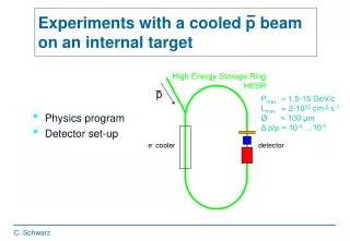
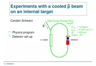
FAIR: Expected antiproton production rate is about 107 1/s The reaction cross-section is about 50 mbarn The limit for mean luminosity: L 107/5·10-26 = 2·1032 cm-2 s-1 High Energy Storage Ring: The ring circumference is about 574 m, revolution period is 2 s life> 104 s 4·1015 cm-2 N 1011 Pellet target
Flux radius Mean distance between pellets Pellet diameter Pellet target = <>thickness
Areal density for Gaussian beam (pellet is in the beam centre) Peak/mean Effective density in cm = 1 mm, = 4·1015 cm-2, Peak/mean = 2.5
The effects leading to the beam heating 1. Scattering on residual gas atoms is negligible if nrg < 109 cm-3 2. Longitudinal heating due to scattering in the target High resolution mode (HR) p ~ 10-4
The effects leading to the beam heating 3. Transverse heating due to scattering in the target 4. Intra-beam scattering In the thermal equilibrium between longitudinal and transverse degrees of freedom in HR (if transverse and longitudinal cooling rates are the same) It is necessary to stabilize the beam emittance at some reasonable level IBS is negligible At
Beam cooling 1. At stochastic cooling one can adjust longitudinal and transverse cooling times independently 2. At electron cooling the cooling times have comparable values for all degrees of freedom D.Reistad et. al., Calculations on high-energy electron cooling in the HESR, Proceedings of COOL 2007, Bad Kreuznach, Germany Intentional misalignment (tilt) of the electron beam is most attractive for stabilization of the emittance value.
Tilt of the electron beam When the misalignment angle reaches a certain threshold value the ions start to oscillate with a certain value of betatron amplitude. Transverse plane Beam profiles Simulations with BETACOOL
VRF V0 t T2 T1 p/p 1 2 s-s0 Compensation of ionization energy loss: barrier RF bucket Compensation of mean energy loss by RF decreases sufficiently requirements to the cooling power max ~ 10-3 V ~ 5 kV
The processes to be simulated 1. Interaction with the pellet target based on realistic scattering models 2. Intra-beam scattering at arbitrary ion distribution 3. Stochastic cooling, taking into account nonlinearity of the force at large amplitudes 4. Electron cooling at electron beam misalignment 5. Longitudinal motion at arbitrary shape of the RF voltage To provide benchmarking Simulations using independent codes (BETACOOL, MOCAC) Comparison with experiments (ESR and COSY) Longitudinal motion in Barrier RF buckets, Investigation of electron cooling with electron beam misalignment, Short term luminosity variation with the WASA pellet target
Physical models of Internal target Longitudinal degree of freedom ; ; n1, n2 – number of excitation events to different atomic energy levels n3 – number of ionization events x – uniform random number Eloss–mean energy loss, x– Gaussian random Estr–energy fluctuations (straggling) N N DP/P0 DP/P0 DP/P0+Estr DP/P DP/P Eloss Eloss
Transverse degree of freedom q – rms scattering angle x – Gaussian random numbers c – screening angle N – number of scattering events x – uniform random numbers target target qstr
s Pelletflux x Average luminosity calculation with BETACOOL code for each model particle Number of events: 1) Integration over betatron oscillation 2) Integration over flux width 3) Number of turns per integration step Number of events for model particle Particle probability distribution Realistic models of interaction with pellet Urban + plural scattering
WASA@COSY experiment For benchmarking BETACOOL code data from COSY experiment (2008 and 2009 runs) was used WASA @ COSY Parameters of COSY experiment
Experiments withoutbarrier bucket h = 8 mm d = 0.03 mm The beam momentum spread can be calculated from measured frequency spread
Investigations of electron cooling at COSY 7-11 April 2010 New fast (~ 40 ms) Ionization Profile Monitor • Measurements of longitudinal component of the cooling force, • Investigation of chromatic instability Possibility to work with Barrier Buckets
Green and yellow lines are signals from pellet counter Blackline is number of particles Other colour lines are signals from different detectors Signals from detectors Simulation of particle number on time Simulation of long scale luminosity on time
Pellet distribution Pellet distribution Effective luminosity calculation Ion beam profile
Short scale luminosity variations Experiment h = 8 mm d = 0.03 mm Simulation h = 0.2 mm d = 0.01 mm
Two variants of detector limit Detector limit Top cut y Average luminosity Average luminosity Full cut y Effective luminosity x
Effective to average luminosity ratio for different detector limit (high-luminosity mode) Top cut Full cut
Effective to average luminosity ratio for different detector limit (high-resolution mode) Top cut Full cut
Conclusions • The choice of the target density depends on the ring acceptance. More strong limitation leading to necessity of the pellet target is RF voltage amplitude • Horizontal beam size at the target has to be stabilized at optimum value (transverse overcooling the beam leads to increase the momentum spread due to IBS and large luminosity variations) • Vertical beam size determines short-scale luminosity variation and optimum value has to be about inter pellet distance) • Current parameters of the beam and target can be optimized. • The code development has to be prolonged as well as experimental study at COSY