Download
1 / 16
160 likes | 291 Views
A Branch-and Bound Algorithm for MDL Learning Bayesian Networks. Jin Tian Cognitive Systems Lab. UCLA. Contents. MDL Score Previous algorithms Search Space Depth-First Branch-and-Bound Algorithm Experimental Results. MDL Score. Training data set: D = {u 1 , u 2 , .. , u N }

E N D
A Branch-and Bound Algorithm for MDL Learning Bayesian Networks Jin Tian Cognitive Systems Lab. UCLA
Contents • MDL Score • Previous algorithms • Search Space • Depth-First Branch-and-Bound Algorithm • Experimental Results
MDL Score • Training data set: D = {u1 , u2 , .. , uN} • Total description length (DL) = length of description of model + length of description of D • MDL principle (Rissanen, 1989):Optimal model minimizes the total description length
G:Graph , U = ( X1 , .. , Xn ) , • DL = DL(Data) + DL(Model) • DL(Model) : Penalty for complexity , # parameters to represent each(i–j) state. • DL(Data|G) : for each case u, use - log P(u|G) as an optimal encoding length (Huffman code) • H term : N * conditional entropy(X|Pa)
Assume: X1 < .. < Xn to reduce search complexity • MDL(G,D) is minimized iff each local score is minimized : Find a subset Pa for each X that minimizes MDL(X|Pa) [here each Parent set can be independently selected.] • For each Xi , sets to search for the Parent set and total of sets.
Previous algorithms • K2: Cooper and Herskovits(1992), BD score • K3: K2 with MDL score • Branch-and-bound: Suzuki(1996) MDL(X|Pa) = H + (log N /2)*K (K= #parameters for parents, H= N*empirical entropy) Adding a node to Pa : K increases by K(old)*(r-1), while H decreases no more than H(old) if H(old) < K : positive MDL and further search is unnecessary • Smaller H for the speed of pruning • lower bound of MDL: MDL >= (log N /2)*K
Search Space • Problem: Find a subset of Uj ={X1 , .. , Xj-1} that minimize the MDL score. • Search space: states-operators set State: a subset of Uj (node) Operator: adding an X (edge) • In a search Tree, a state T with l variables is {Xk1, .. , Xkl } where Xk1 < .. < Xkl are ordered. (Tree order). A legal operator: Adding a single variable after Xil .
(A serach for the parents of X5 ) • The search tree for Xj has 2j-1 nodes and the tree depth is j-1
Branch-and-BoundAlgorithm • In finding a parent of Xj , assume we are visiting a state T = {.., Xkl} and let W be the set of rest variables. We want to decide if we need to visit the branch below T’s child : T {Xq}, Xq W . • Pruning: Find initial minMDL from K3 (speedy) and compare with the lower bound of MDL of that branch.
Lower bound (Suzuki): • Better lower bound: • Pruning: If , all branches below T {Xq} can be pruned.
In node ordering: Xk1 < .. < Xk(j-1) , Xk1 appears least, Xk(j-1) appears most. • Tree Order as: H(Xj|Xk1)<= H(Xj|Xk2)<= .. <=H(Xj|Xk(j-1)) • Result: Most of the lower bounds have larger values. Visiting of fewer states.
Empirical Results • ALARM(37 nodes, 46 edges) • Boerlage92(23 nodes, 36 edges) • Car-Diagnosis_2(18 nodes, 20 edges) • Hailfinder2.5(56 nodes, 66 edges) • A(54 nodes, dence edges) • B(18 nodes 39 edges)