Download
1 / 64
640 likes | 646 Views
Visualization. Chapter 12. Introduction: In this chapter, we apply almost everything we have done so far to the problem of visualizing large data sets that arise in scientific and medical applications. Fortunately, we can bring many tools to bear on these problems

E N D
Visualization Chapter 12
Introduction: • In this chapter, we apply almost everything we have done so far to the problem of visualizing large data sets that arise in scientific and medical applications. • Fortunately, we can bring many tools to bear on these problems • We can create geometric objects • We can color them, animate them, or change their orientation. • With all these possibilities, and others, there are multiple ways to visualize a given data set, and we will explore some of the possibilities in this chapter. Chapter 12 -- Visualization
1. Data + Geometry • Data comprise numbers. • They are not geometric objects and thus they cannot be displayed directly by our graphics systems. • Only when we combine data with geometry are we able to create a display and to visualize the underlying information. • A simple definition of (scientific) visualization is: • the merging of data with the display of geometric objects through computer graphics Chapter 12 -- Visualization
We consider three types of problems: • scalar visualization: • we are given a three-dimensional volume of scalars, such as X-ray densities. • vector visualization: • we start with a volume of vector data, such as the velocity at each point in a fluid • tensor visualization: • we have a matrix of data at each point, such as the stresses within a mechanical part. Chapter 12 -- Visualization
We must confront several difficulties • One is the large size of the data sets. • Many of the most interesting applications involve data that are measured over three spatial dimensions and often also in time. • For example, the medical data such as from an MRI can be at a resolution of 512 x 512 x 200 points. • The visible-woman data set is a volume of densities that consist of 1734 x 512 x 512 data points. • consequently, we cannot assume that any operation on our data, no matter how conceptually simple it appears, can be carried out easily Chapter 12 -- Visualization
Second, these data are only data • They are not geometric objects • Thus we must translate these data to create and manipulate geometric objects. • Third, we may have multidimensional data points • For example, • When we measure the flow of a fluid at a point, we are measuring the velocity, a three-dimensional quantity. • When we measure the stress or strain on a solid body at some internal point, we collect a 3x3 matrix of data. • How we convert these data to geometric objects and select the attributes of those objects determines the variety of visualization strategies. Chapter 12 -- Visualization
2. Height Fields and Contours • One of the most basic and important tasks in visualization is visualizing the structure in a mathematical function. • This problem arises in many forms, the biggest difference is • how we are given the function • implicitly, explicitly, or parametrically. • And in how many independent variables define the function. Chapter 12 -- Visualization
In this section, we consider two problems that lead to similar visualization methods • One is the visualization of an explicit function of the form: • z = f(x,y) • with two dependent variables • Such functions are sometimes called height fields Chapter 12 -- Visualization
The second form is an implicit function in two variables: • g(x,y) = c • where c is a constant. • This equation describes one or more two-dimensional curves in the x,y plane. There may also be no x,y values that satisfy the equation. • This curve is called the contour curve, corresponding to c Chapter 12 -- Visualization
2.1 Meshes • The most common method to display a function f(x,y) is to draw a surface. • If the function f is known only discretely, then we have a set of samples or measurements of experimental data of the form: • zij = f(xi,yj) • We assume that the data are evenly spaced. • If f is known analytically, then we can sample it to obtain a set of discrete data with which to work. Chapter 12 -- Visualization
One simple way to generate a surface is through either a triangular or a quadrilateral mesh. • Thus the data define a mesh of either • NM quadrilaterals or • 2NM triangles. • The corresponding OpenGL programs are simple. • The following figure shows a rectangular mesh from height data for a part of Honolulu, Hawaii Chapter 12 -- Visualization
There are interesting aspects to and modifications we can make to the OpenGL program • First, if we use all the data, the resulting plot may contain many small polygons • The resulting line density may be annoying and can lead to moiré patterns • Hence we might prefer to sub-sample the data • use every kth point for some k • or by averaging groups of data to obtain a new set of samples with smaller N and M. Chapter 12 -- Visualization
Second, the figure we saw was drawn with both black lines and white filled polygons. • The lines are necessary to display the mesh. • The polygons are necessary to hide data behind the mesh. • If we display the data by first drawing the polygons in back and then proceed towards the front, the front polygons automatically hide the polygons further back. • Since the data is well-structured, this is possible. • If hidden surface removal is done in software, this might be faster than turning on z-buffering. Chapter 12 -- Visualization
There is one additional trick that we used to display this figure. • If we draw both a polygon and a line loop with the same data, such as: • glcolor3f(1.0,1.0,1.0); • glBegin(GL_QUADS) • ...glVertex3i(...) • glEnd(); • glColor3f(0.0,0.0,0.0); • glBegin(GL_LINE_LOOP); • ...glVertex3i(...) • glEnd(); • then the polygon and the line loop are in the same plane. Chapter 12 -- Visualization
Even though the line loop is rendered after the polygon, numerical inaccuracies in the renderer often cause part of the line loop to be blocked by the polygon. • We can enable the polygon offset mode and se the offset parameter as in: • glEnable(GL_POLYGON_OFFSET_FIL) • glPolygonOffset(1.0, 0.5) • These functions move the lines slightly toward the viewer relative to the polygon, so all the desired lines are now visible. Chapter 12 -- Visualization
The basic mesh plot can be extended in many ways. • If we display only the polygons then we can add lighting to create a realistic image of a surface in mapping applications. • The required normals can be computed from the vertices of the triangles or quadrilaterals. • Another option is to map a texture to the surface • The texture map might be an image of the terrain from a photograph or other information that might be obtained by digitization of a map. • If we combine these techniques, we can generate a display in which, by changing the position of the light source, we can make the image depend on the time of day. Chapter 12 -- Visualization
2.2 Contour Plots • One of the difficulties with mesh plots is that, although they give a visual impression of the data, it is difficult to make measurements from them. • An alternative method of displaying the height data is to display contours -- curves that correspond to a fixed value of height. • We can use this method to construct topographic maps used by geologists and hikers. • The use of contours is still important, both on its own and as part of other visualization techniques. • We solve the accuracy problem of sampled data by using a technique called marching squares Chapter 12 -- Visualization
2.3 Marching Squares • Suppose: • we have a function f(x,y) that we sample at evenly spaced points on a rectangular array (or lattice) in x and y. • that we would like to find an approximate contour curve • Our strategy is to construct a curve of connected line segments (piecewise linear) • We start with a rectangular cell determined by four grid points Chapter 12 -- Visualization
Our algorithm finds the line segments on a cell-by-cell basis using only the values of z at the corners of the cell to determine whether the desired contour passes through the cell. • Consider this case Chapter 12 -- Visualization
Then the contour line will go through the box, similar to the figure below. • The principle to consider is: • When there are multiple possible explanations of a phenomenon that are consistent with the data, choose the simplest one. Chapter 12 -- Visualization
Returning to our example: • We can now draw the line for this cell. The issue is where do we draw it? • Pick the mid point on each edge and connect them • Interpolate the crossing points. • There are 16 (24)ways that we can color the vertices of a cell using only black and white. • All could arise in our contour problem. • These cases are itemized on the next slide Chapter 12 -- Visualization
If we study these cases, we see that there are two types of symmetry • Rotational (1 & 2) • Inverses (0 & 15) • Once we take symmetry into account, only 4 cases truly are unique: Chapter 12 -- Visualization
The first case has no line • The second case is what we just discussed. • The third case has a line from side to side • The fourth case is ambiguous since there are two equally valid interpretations Chapter 12 -- Visualization
We have no reason to prefer one over the other • so we could pick one at random. • Always use only one possibility • ... • But as this figure shows, we get different results depending upon the interpretation we choose Chapter 12 -- Visualization
Another possibility is to subdivide the cell into four smaller cells, • and then draw our lines. • The code is fairly simple: • int cell(double a, double b, double c, double d) • { • int num=0; • if(a>THRESHOLD) num+=1; • if(b>THRESHOLD) num+=8; • if(c>THRESHOLD) num+=4; • if(d>THRESHOLD) num+=2; • return num; • } Chapter 12 -- Visualization
We then can assign the cell to one of the four cases by: • switch(num){ • case 1: case 2: case 4: case 7: case 8: • case 11: case 13: case 14: • draw_one(num, i,j,a,b,c,d); • break; // contour cuts off one corner • case 3: case 6: case 9: case 12: • draw_adjacent(num,i,j,a,b,c,d); • break; // contour crosses cell • case 5: case 10: • draw_opposite(num, i, j, a,b,c,d); • break; // ambiguous cases • case 0: case 15: • break; // no contour in cell • } Chapter 12 -- Visualization
void draw_one(int num, int i, int j, double a, double b, • double c, double d) { • // compute the lower left corner of the cell and s_x and s_y here. • switch(num){ • case 1: case 14: • x1=ox; y1 = oy+s_y; • x2= ox+s_x; y2 = oy; • break; • /* the other cases go here • case 2: case 13: ... • case 4: case 11: ... • Case 7: case 8: ... • } • glBegin(GL_LINES); • glVertex2d(x1,y1); • glvertex2d(x2,y2); • glEnd(); • } Chapter 12 -- Visualization
The following figure shows two curves corresponding to a single contour value for: • f(x,y) = (x2+y2+a2)2-4a2x2-b4 (with a=0.49, b=0.5) • The function was sampled on a 50x50 grid • The left uses midpoint, the right interpolation. Chapter 12 -- Visualization
This next figure shows the Honolulu data set with equally spaced contours: • The Marching squares algorithm just described is nice because all the cells are independent. Chapter 12 -- Visualization
3. Visualizing Surfaces and Scalar Fields • The surface and contour problems just described have three-dimensional extensions. • f(x,y,z) defines a scalar field. • An example is the density inside an object or the absorption of X-rays in the human body. Chapter 12 -- Visualization
Visualization of scalar fields is more difficult than the problems we have considered so far for two reasons: • First, three-dimensional problems have more data with which we must work. • Consequently, operations that are routine for 2D data (reading files and performing transformations) present practical difficulties. • Second, when we had a problem with two independent variables, we were able to use the third dimension to visualize scalars. • When we have three, we lack the extra dimension to use for display. • Nevertheless, if we are careful, we can extend our previously developed methods to visualize three-dimensional scalar fields Chapter 12 -- Visualization
3.1 Volumetric Data Sets • Once again, assume that our samples are taken at equally spaced points in x,y, and z • The little boxes are called volume elements or voxels Chapter 12 -- Visualization
Even more so than for two-dimensional data, there are multiple ways to display these data sets. • However there are two basic approaches: • Direct Volume Rendering • makes use of every voxel in producing an image • Isosurfaces • use only a subset of the voxels Chapter 12 -- Visualization
3.2 Visualization of Implicit Functions • This is the natural extension of contours to 3D • Consider the implicit function in three dimensions • g(x,y,z) = 0 where g is known analytically. • One way to attack this problem involves a simple form of ray tracing (ray casting) Chapter 12 -- Visualization
Finding isosurfaces usually involves working with a discretized version of the problem • replacing g by a set of samples taken over some grid. • Our prime isosurface visualization method is called marching cubes, the three-dimensional version of marching squares. Chapter 12 -- Visualization
4. Isosurfaces and Marching Cubes • Assume that we have a data set, where each voxel is a sample of the scalar field f(x,y,z) • Eight adjacent grid points define a three-dimensional cell as shown here: Chapter 12 -- Visualization
We can now look for parts of isosurfaces that pass through these cells, based only on the values at the vertices. • There are 256=28 possible vertex colorings, but once we account for symmetries, there are only 14 unique cases Chapter 12 -- Visualization
Using the simplest interpretation of the data, we can generate the points of intersection between the surface and the edges of the cubes by linear interpolation. • Finally we can use the triangle polygons to tessellate these intersections. Chapter 12 -- Visualization
Because the algorithm is so easy to parallelize and, like the contour plot, can be table driven, marching cubes is a popular way of displaying three-dimensional data. • There is an ambiguity problem analogous to the one for contour maps Chapter 12 -- Visualization
5. Mesh Simplification • On disadvantage of marching cubes is that the algorithm can generate many more triangles than are really needed to display the isosurface. • One reason can be the resolution of the data set. • We can often create a new mesh with far fewer triangles such that the rendered surfaces are visually indistinguishable. • There are multiple approaches to this mesh simplification problem Chapter 12 -- Visualization
One popular approach is triangle decimation. • It seeks to simplify the mesh by removing some edges and vertices. • Example: • The decision as to which triangles are to be removed can be made using criteria such as the local smoothness or the shape of the triangles • The latter is important since long thin triangles do not render well Chapter 12 -- Visualization
Other approaches are based upon resampling the surface generated by the original mesh , thus creating a new surface • Probably the most popular technique is Delauney triangulation. • This algorithm creates a triangular mesh in which the circle determined by the vertices of each triangle contains no other vertices. • The complexity of this is O(n log n) Chapter 12 -- Visualization
6. Direct Volume Rendering • The weakness of isosurface rendering is that not all voxels contribute to the final image. • Consequently, we could miss the most important part of the data by selecting the wrong isovalue. • Direct volume rendering constructs images in which all voxels can make a contribution to the image. Chapter 12 -- Visualization
Early methods for direct volume rendering treated each voxel as a small cube that was either transparent or completely opaque. • These techniques produced images with serious aliasing artifacts. • With the use of color and opacity, we can avoid or mitigate these problems. Chapter 12 -- Visualization
6.1 Assignment of Color and Opacity • We start by assigning a color and transparency to each voxel. • If the data are from a computer-tomography scan of a person’s head, we might assign colors based upon the X-ray density. • Soft tissues (low density) might be red. • Fatty tissues (medium densities) might be blue • Hard tissues (high densities) might be white • Empty space might be black. Chapter 12 -- Visualization
Often, these color assignments are based upon the voxel distribution • Here is an example histogram Chapter 12 -- Visualization
6.2 Splatting • Once colors and opacities are assigned,, we can assign a geometric shape to each object. • Sometimes this is done with a back to front painting. • Consider the voxels in the following figure Chapter 12 -- Visualization
Each voxel is assigned a simple shape and this shape is projected onto the image plane. This projected footprint is also known as a splat. • Color plate 28 is an example of this Chapter 12 -- Visualization
6.3 Volume Ray Tracing • An alternative direct-volume rendering technique is front-to-back rendering by raytracing. Chapter 12 -- Visualization