Download

1 / 76
760 likes | 766 Views
Algorithms for Image Matching for Visual Robot Navigation. Ilan Shimshoni University of Haifa. Visual Homing. Ronen Basri Ehud Rivlin Ilan Shimshoni ICCV98 IJCV99. Robot Navigation Traditional Approach. Step 2.5 meters north-west and turn right by 10 degrees.

E N D
Algorithms for Image Matchingfor Visual Robot Navigation Ilan Shimshoni University of Haifa
Visual Homing Ronen Basri Ehud Rivlin Ilan Shimshoni ICCV98 IJCV99
Robot NavigationTraditional Approach Step 2.5 meters north-west and turn right by 10 degrees Fixed environment, measured carefully in advance.
Alternativeapproach: Make the robot see! Mount a camera on the robot, give it an image taken from the target pose, and let the robot navigate to the target.
Source Target (Sisley)
Algorithm Current image Target image Correspondence Epipolar geometry Handle missing parameters Step toward the target
Major Challenges in image feature matching • Match features • Deal with wide baseline images • Deal with many incorrect matches (outliers) • Accurately compute the epipolar geometry • Deal with degenerate point configurations (e.g. planar surfaces) • Deal with changes in the illumination
Talk Outline • Short overview of several papers • Accurate estimate of epipolar geometry • New robust estimation method • Matching outdoor images taken at different lighting conditions • Dealing with wide baseline images with very high percentages of outliers. • The BEEM algorithm
Motion Recovery by Integrating over the Joint Image Space Liran Goshen Ilan Shimshoni Daniel Keren P. Anandan ICCV 2003, IJCV 2005
The fundamental matrix • Algebraic representation of the epipolar geometry • Projective mapping from points to lines • Correspondence condition • F has 7 d.o.f. i.e. 3x3-1(homogeneous)-1(rank2)
Fundamental Matrix Estimation • The algebraic method • The Sampson method • The normalized 8 point method • The geometric method
The Geometric Method X belongs to the joint image space F defines a manifold in the JIS
The Geometric Method X belongs to the joint image space F defines a manifold in the JIS
Integrated Maximum Likelihood We have to integrate over the ‘nuisance’ parameters, yielding Joint Gaussian pdf • JIS -> fitting manifold to data measured. • IML- seeks the manifold which has the highest “support”.
Contributions • The geometric method is not the “goldan standard” • Yields superior results for small motions seperates rotation from translation • Good when the moving object occupies only a small part of the image • Slow
Projection Persuit based M-Estimator (pbM) • Hifeng Chen & Peter Meer, ICCV 2003 • Stas Rozenfeld & Ilan Shimshoni, CVPR 2005 • R. Subbarao & Peter Meer, CVPR 2005
RANSAC- RANdom SAmple Consensus • While i < sample_count • Randomly select a sample of s data points. • Instantiate the model from this subset. • Determine the number of inliers. • The model with the largest consensus set is selected. • The model is re-estimated using all the inliers.
Demonstration of Projection Pursuit Based M-Estimator example 1 : sample 2 points and compute the model
Demonstration of Projection Pursuit Based M-Estimator example 1: compute pbM-Estimator
Demonstration of Projection Pursuit Based M-Estimator example 1: compute density
Demonstration of Projection Pursuit Based M-Estimator example 1: decide which points are inliers and correct the model
Demonstration of Projection Pursuit Based M-Estimator example 1 - results
Demonstration of Projection Pursuit Based M-Estimator example 2
Demonstration of Projection Pursuit Based M-Estimator example 2
Demonstration of Projection Pursuit Based M-Estimator example 2
Demonstration of Projection Pursuit Based M-Estimator example 2
Demonstration of Projection Pursuit Based M-Estimator example 2
Demonstration of Projection Pursuit Based M-Estimator example 3
Demonstration of Projection Pursuit Based M-Estimator example 3
Demonstration of Projection Pursuit Based M-Estimator example 3
Demonstration of Projection Pursuit Based M-Estimator example 3
Demonstration of Projection Pursuit Based M-Estimator example 3
Advtantages • No user supplied scale parameter • Uses the distribution of errors to separate between inliers and outliers • Can be adapted for geometric distances. Has been used for matching 3D data to parameterized surfaces contaminated with large amounts of outliers
Image Matching UsingPhotometric Information Michael Kolomenkin Ilan Shimshoni CVPR 2006
The goal • Many matching algorithms exist however they may fail in severe conditions • wide baseline • changes in illumination • Most existing techniques are based on geometric features • Our method employs color information to improve performance
The Alchemist • Making gold out of led • Apply segmentation to the two images (Edison) • Match image features (SIFT) • Both have problems: • The segmentation results in the two images are not consistent. Over & under segmentation • The percentage of incorrect matches is very high • Combine them to yield quality results
Intensity invariant color space Macbeth chart cells under 30 different illuminants:
( ( ( ) j ( ) j ( ) ) ( ) ) ~ ~ f f G A A B B G B A G B ¢ T G A ¢ T + + ¢ ¢ c c = = 0 0 0 0 0 0 0 0 ; ; Group matching • Segment matching definition. • Illumination varies slowly over image. B B1 ΔT ΔT A4 B3 A1 B0 ΔT A0 ΔT B2 A3 ΔT A2 R
Adding point features • From our method – Pr(Si = Sj) for every i, j. • From other application (SIFT) – {F1,F2}k with Pr({F1,F2}k). • Using Bayesian approach the probabilities are updated. F1 F2 S1 S2
Results Original SIFT 14 - 37 Outliers Inliers Our method 14 - 4
Results Original SIFT 32 - 38 Outliers Inliers Our method 32 - 7
Guided Sampling via Weak Motion Models and Outlier Sample Generation for Epipolar Geometry Estimation Liran Goshen Ilan Shimshoni CVPR 2005
When to stop the algorithm? The number of iterations is chosen sufficiently high to ensure with probability, p, that at least one of sample is free from outliers. є is not generally known in advance. The number of samples drawn in RANSAC is higher than predicted from the mathematical model.
Weak motion model • In general each point in the first image moves to its corresponding epipolar line. • We used an affine transformation as a WMM, i.e., • Three points in the joint image space define a unique affine transformation.
Weak motion model • We use an affine transformation that has been formed from three inlier correspondences as a WMM. • Let {wi} be as set of Nw WMMs. • This median distance can be thought of as a random variable and is modeled as a mixture model: where
Weak motion model N=411 Nin=59 ε=0.86
Probability estimation The probability , , that correspondence is an inlier can be calculated by • Non-parametric estimation. • Inlier distances bounded by an unknown parameter D.
Outlier sample The estimation of is more problematic. We have tried three methods to generate the outlier sample: • Uniformly • Corner based • Algorithm guided
Outlier sample • Algorithm guided X