Download
1 / 36
380 likes | 531 Views
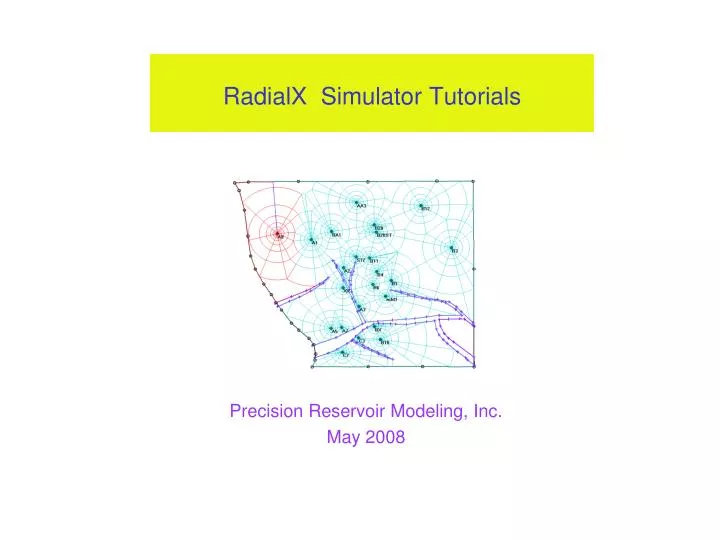
RadialX Simulator Tutorials. Precision Reservoir Modeling, Inc. May 2008. Introduction to the tutorial.

E N D
RadialX Simulator Tutorials Precision Reservoir Modeling, Inc. May 2008
Introduction to the tutorial • Sections 1 to 4 instruct users to create, modify, run and review results of a simple box-like reservoir model with a couple of wells from scratch. Steps involved in this process are mainly specifying PVT properties, rock properties, reservoir geometry, well locations, well perforations, and well control. • A simulation model could be more complicated because of its irregular boundary, faults, and complicated wellbore completions. Section 5shows how to handle complicated wellbore completions, load in reservoir structure and property data of ZMAP/Bitmap or Corner point grid formats. This section also shows how to modify reservoir boundary/faults and well locations, and manipulate the simulation grid.
Outlines 1. Project Input and settings 1.1 Set working folder 1.2 Set project start time 1.3 Edit PVT properties 1.4 Edit rock properties 1.5 Add reservoirs 1.6 Add wells • Create grid model 2.1 Structure view 2.2 Gridding parameters 2.3 Grid 3D view and map operations 2.4 Comments about simulation model 2.5 Modify cell values on property table 2.6 Modify cell values in 3D view • Run the model • Review results and save files 4.1 Chart view 4.2 3D map view 4.3 Table view 4.4 Save files • Add complexities to your model 5.1 Reservoir data of corner point grid format 5.2 Reservoir data of bitmap/ZMAP format 5.3 Manipulate model grid 5.4 Fractured horizontal/vertical wells 5.5 Gridding for horizontal well, fractured horizontal/vertical well 5.6 Template for fractured horizontal well
1. Project Input and settings1.1 Set working folder Note: A simulation project requires the user to click on these menu items one by one to perform these tasks: a)File to create, open, save and close case files; b)Settings for project settings; c)Fluids for editing PVT tables; d)Rocks for editing rock property table; e)GridModel for reservoir structure/property, well data and simulation grid; f)RunModel for executing the simulation runs; and g)ViewResults for reviewing results. 1.1.1 Start RadialX Simulator program and click the File New menus in the main window to bring up the Start A Case window 1.1.2 Click Browse command button directs user to the working folder and provide a case name for your simulation project 1.1.3 Click OK button to go to the next step
1.2 Set project start time Note: Model features can be specified in the Model Spec tab, such as sorption, compaction, non-Darcy flow, compositional/thermal, dual porosity, and dual permeability. 1.2.1 Click on Setting menu to bring up the Project Setting window. 1.2.2 Specify simulation start time. During a simulation run, the simulator checks model data integrity and does calculations, starting from this time. Put any note here
1.3 Edit PVT properties 1.3.1 Click Fluids menu to bring up the Fluid Properties window to edit PVT tables 1.3.2Add PVT tables one by one by clicking Actions Add Fluid Table menus to bring up the following Fluid Properties window. If your PVT data are stored in text files, please click Load from file menu and follow the directions.
1.3 Edit PVT properties -- continued 1.3.3 Click a tab to select table to view and edit Note: Correlations are provided to generate PVT table 1.3.4 Click each column header to view particular chart Note: For any spreadsheet in the simulator, double click on a cell to type data in; use Ctrl_C/Ctrl_X/Ctrl_V to copy/cut/paste data.
1.4 Edit rock properties 1.4.1 Click Rocks menu to bring up the Rock Properties window 1.4.2Add rock property table one by one by clicking Actions Add Rock Table menus. If your rock data are stored in text files, please click Load from file menu and follow the directions.
1.4 Edit rock properties -- continued 1.4.3 Click each tab to select the set of data to specify. The non-Darcy flow parameters are specified in General Data tab. If users checked sorption or compaction options in Project Settings window, the corresponding data tab will show up here
1.4 Edit rock properties -- continued 1.4.4 Click each tab to input the table data, or generate table using the correlations provided .
1.5 Add reservoirs 1.5.1 In the main window, click the GridModel menu to start the editing process by bring up the following Model & Results window
1.5 Add reservoirs - continued Note: Highest and lowest elevation values of reservoir structure will be calculated later by simulator. 1.5.2 Right click GridModel node, then click Add Reser/Sand to bring up the Reservoir Structure/Property window to add a reservoir. If there is no existing reservoir, the window on the right will jump up automatically. 1.5.3 Choose Simple Geometry option for reservoir structure 1.5.4 Select Rectangular to generate a box like reservoir
1.6 Add wells 1.6.2 For a vertical well, onlyspecify name, x and y coordinates; for an angled well, also provide the wellbore deviation data in the Deviation Survey tab screen 1.6.1 Right click Wells node, then click Add Well to bring up the Well Details window. Add well one by one to your simulation model Note: The Activation Time and Abandon Time are for dynamic gridding, telling simulator to redo gridding, when a well is activated or abandoned. Leave them blank, if you do not consider dynamic gridding 1.6.3 Specify well completion data in the WellboreCompletions tab screen. Note: Perforations can be specified as layer to layer, MD to MD, or TVD to TVD
1.6 Wells – continued -- Add first well: Prod1 Note: Oil rate is set to be the default simulation driver for a well. You may click the cell and change it 1.6.4 In the Production Schedule Tab screen, input production history data in the spreadsheet. Note: Well control logics can be input in Well Constraints tab screen.
1.6 Wells – continued -- Add second well: Prod_Inj Note: The only thing different for this well is: it produces oil at 650 BOPD from day 0 to 100, and injects water at 1050 BWPD from day 100 on.
2. Create grid model 2.1 Structure view Note: The function of each item in the tool bar can be found by moving mouse pointer over it. You can add wells, set or change reservoir boundary, and perform other functions in 3D view 2.1.1 Click the Load node will couple wells to the reservoir. The simulator will detect how the wells intersect the reservoir for gridding purpose and show a 3D view of the reservoir. Note: After adding the Rect reservoir, Prod1well, and Prod_Inj well, the left pane of the window will look like this, when expanding all the tree nodes. Note: If reservoir structure/property data is in ZMAP/corner point grid format or digitized bitmap, the structure map will show here, and the related property node will be added under the Structure/Prop folder on the left pane. Click on the property node will show its property map view. The I-J values and cell values will show, from top to bottom layers, by clicking the cell on the map, with Shift key holding.
2.2Gridding parameters 2.2.1 Click on the 3D gridding Button to bring up the 3D gridding window 2.2.2 Take default values or change them on the Areal Gridding screen Circle number around wellbore, with the first circle being wellbore itself Allowed angle degree between radii in the same wellbore If Manual box is checked, the circles provided in this spreadsheet will be used for gridding. If Re Multiplier is 1.0, the whole outmost circles from all wellbores are supposed to cover every corner of the reservoir. These circles have the same size. Circles distribution will be different, as it changes. If the area of a boundary cell is smaller than this criterion value, it will not be counted.
2.2 Gridding parameters -- continued 2.2.3 In the Vertical Gridding tab, specify the way you want to vertically divide the reservoir. Note: gridding can be set for each geological layer (simple geometry reservoir only has one layer). If you choose Proportionally Divide, please provide the setting in the spreadsheet, e.g. 20, 30, and 50.
2.2 Gridding parameters -- continued 2.2.4 Click the DoGridding menu to generate the simulation grid Note: If you want to give grid cells uniform values in each layer during gridding, provide the values and check this box. Note: Click ViewGrid menu, if you only want to view existing grid wireframe. The following grid wire frame will show up, if already existing.
2.3Grid 3D view and operations Note: 3D grid wireframe will show up, when the gridding process is done. 3D Map Operations: Press and move left mouse button will turn around the map; press and move the right mouse button will change the view size; hold CtrL key down, press mouse button, and drag will translate the map. Click it to view other layers. Note: model data can be viewed, by clicking the linked tree node
2.4 Comments about simulation model • By now the simulation grid has been setup for the reservoir. Each grid cell has its property values. Perforations and rate history are also specified for each well. Therefore, your model is complete and ready for simulation runs. The following Sections 2.5 and 2.6 show how to modify, when needed, the cell property values on the property table or 3D map. • In the table approach, you may specify the new value, well range, and IJK range for the modification. This is also the place you initialize the model using hydraulic and capillary pressure equilibrium. • In the 3D map approach, you can click on a cell to bring up the cell property values at that location. You then specify the new value, the well range, and IJK range for the modification. • In RadialX Simulator, each grid cell belongs to a well domain. • All your actions of initializing and modifying the model are recorded for future review.
2.5 Modify cell values on property table Note: all the actions you have taken to modify cell values are recorded by the simulator and can be reviewed by clicking ModelHistory menu. 2.5.1 Click the Initialization node will bring up the Cell Values window 2.5.2 You can modify cell values by choosing well range, IJK range, property type, new value and clicking Modify button Note: If you provided GOC/WOC data in rock property tables, you can initialize model using equilibrium method.
2.6 Modify cell values in 3D view Note: You may also select property type and K range by clicking and dragging in spreadsheet The spreadsheet will go away if Done button is clicked. 2.6.2Press and hold the Shift key, click a cell in the view will bring up the above spreadsheet and display the values of the cells in that location (top to bottom) 2.6.1 Click a property node here to view it in 3D 2.6.3 You may further specify property type, well range, IJK range, new value and click Modify button to modify model. Or modify in spreadsheet cells directly Click here to view values of different layers Click here to change color scale
3. Run the model 3.3 Click the Execute menu to start the model run. 3.1 Click the RunModel menu in the main window to bring up the RunModel window. When run is started, the simulator first checks model integrity. If fatal errors are found, the run will be stopped; if non-fatal issues are found, they will be displayed at the Case Diagnostic screen and you can decide to continue or stop the run; if every thing goes well, the run will automatically continue. 3.2. Specify the maximum allowed time step number and the simulation stop time. During model run, if you want to “take pictures” of property value distribution at different times, specify the frequency and the maximum allowed “picture” number.
4. Review results and save files 4.1. Click ViewResults menu in the main window to bring up the Model & Results window to review the simulation results.
4.1 Chart view 4.1 Click a node to see the result linked to it. To show the values of a line point, click the line to highlight it, then click the point. Results are classified as reservoir level (in the Rect folder) and well level (in the Wells Charts folder). Click any node to view the linked results. Click x or y axes to change graph scale.
4.2 3D map view Click it to go to next “picture”. Click it to change map layer. Press and hold the Shift key, click a cell will bring up a spreadsheet and display the values of the cells in that location (top to bottom) at picture time. 4.2.1 Click a sub-node of 3-D View folder to view that property value map in 3D.
4.3 Table view 4.3.1 Click Table View node to view that property values at “picture” time.
4.4 Save files 4.4.1. Click Save or Save As menu to save your model data and simulation results. 4.4.2. Click Close menu to terminate the simulation application.
5. Add complexities to your model5.1 Reservoir data of corner point grid format 5.1.1 If you have reservoir structure and property data in corner point grid format, check this button in the Reservoir Structure/Property window. 5.1.2 Click Add file entry button to add data file into list one by one.
5.2 Reservoir data of bitmap/ZMAP format If you have property maps, click the Property menu and follow the same procedure as you treated the structure maps. 5.2.2 Click one of these buttons to specify the layer surface one by one. They can be surface structure map, isopach map, pane of equal elevation, or pane of equal distance from the above surface. The first item in the list must be a surface structure map. 5.2.6 Click Mapping menu to set the sampling grid and to interpolate for structure and property values, after all bitmaps have been digitized. 5.2.1 Select the Build from ZMAP or Bitmap button in Reservoir Structure/Property window. 5.2.3 If an item in the Horizon list is a bitmap file, you need click this button to bring up the following Digitize Bit Map widow to digitize it.
5.2 Reservoir data of bitmap/ZMAP format -- continued 5.2.5To add a well, move mouse to a well location and right click it to bring up the context sensitive menu, then click Add Well menu. A well will be added at that location; To add contour, fault or reservoir boundary lines, please click the corresponding item in the context sensitive menu, then trace the line by left mouse clickings. When you come to the last tracing point, double click the left button to end the line tracing. To enlarge view, click ViewEnlargeView menus, then select the region to be enlarged by mouse click, drag and release. To restore view, click View -> RestoreView menus. To modify an exiting digitized object, press Shift key, mouse click on it, and drag. The object can be wells, line points or segments. 5.2.4 To digitize a bit map, you first set the map coordinates by specifying two reference marks on the map: move mouse pointer to a reference mark and right click to bring up the context sensitive menu, then click Set Benchmark A and provide the x and y coordinates. Follow the same steps for the second reference mark.
5.3 Manipulate model grid User can modify boundary/fault line and well location by pressing the Shift key, mouse clicking on the subject and dragging it. 5.3.1 If user clicks ArealGrid node, the Reservoir and ArealGrid window will come up. Right clicking on an item on the map will bring up the context sensitive menu. You then can choose different things to do. 5.3.2 Click Grid menu and then choose ViewGrid or DoGridding menu. Note: User is encouraged to first test the gridding parameters here before 3D gridding operation. The Add Grid Line function is only available in this window. To add a grid line to a well, right click the well to bring up the context sensitive window, then click Add Grid Line menu, then move mouse to lead the line from the well to boundary/fault, and mouse click on boundary/fault. The added line will be shown in blue. Re-do the gridding to incorporate the added line into the grid.
5.4 Fractured horizontal/vertical wells Specify well type as “Angled” for horizontal well. If a wellbore has fractures, specify its MD and other parameters for each individual fracture along with deviation survey data. 5.4.1 Click the well node to bring up the Well Details window to specify wellbore/fracture data, etc. Fractures may have its own rock property table to specify relative perm, capillary pressure, variation of perm and compressibility with enclosure pressure, etc.
5.5 Gridding for horizontal well, fractured horizontal/vertical well User may check the Manual Circle box to add/adjust circle radii in the spreadsheet. If this box is unchecked, RadialX will automatically figure out the right circle radii. For fractured horizontal well, one of the radius will be made equal to fracture half length. 5.5.1 For Angled well and fractured vertical well, please place an inner disc region around the wellbore or fracture for gridding. For a horizontal well, the elliptical grid around wellbore is generated by evenly distributing a number of gridding points along the wellbore: Control Point interval set the interval between control points; but total point number cannot exceed Max Control Point No. If there are hydraulic fractures on the wellbore, a number of locally refined grid lines will be placed around each fracture. For fractured vertical well, these two parameters specify how many elliptical circles will be placed within the inner disc region, and how many divisions along fracture half wing.
5.6 Template for fractured horizontal well 5.6.1 When setting up reservoir structure, user may select Simple Geometry -> Rectangular/Horizontal Well to access the template. Then further change wellbore/fracture parameters in Well Detail window. If choosing this gridding option, elliptical circles will be placed around wellbore in X-Y plane and cast down in Z direction. If choosing this gridding option, circles will be placed around wellbore in X-Z plane and cast down in Y direction.