Download
1 / 7
150 likes | 504 Views
Rayleigh-Taylor instabilities (with animations).

E N D
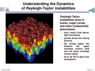
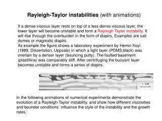
Rayleigh-Taylor instabilities (with animations) If a dense viscous layer rests on top of a less dense viscous layer, the lower layer will become unstable and form a Rayleigh Taylor instability. It will rise through the overburden in the form of diapirs. Examples are salt domes or magmatic diapirs. As example the figure shows a laboratory experiment by Hemin Koyi (1989, Dissertation, Uppsala) in which a light layer (PDMS,black) was overlain by a denser layer (bouncing putty). The faulted basement (plastillina) was camparably stiff. After centrifuging the buoyant layer becomes unstable and forms a series of diapirs. In the following animations of numerical experiments demonstrate the evolution of a Rayleigh-Taylor instability, and show how different viscosities and boundar conditions influence the style of the instability and the growth rates.
Model set up Boundary condition: Free slip , no slip Density: 1 (kg/m3) Viscosity: 1 (Pa s) Gravity 1 (m/s2) h: 1 (m) Symmetric at the sides Perturbation 0.01 or 0.03 (m) 0.1 (m) Density: 0 (kg/m3) Viscosity: 0.01, 1, 100 (Pa s) Free slip , no slip
A Definitions: Growth rate describes the growth of a perturbation of initial amplitude A0: Characteristic wavelength char: A perturbation with this wavelenth is growing fastest Dominant wavelength: This wavelength dominates the final stage (often equal to the char. wavelenth, but sometime inherited from the initial wavelength)
Case 1: Same viscosities Free slip Total run time: 4000 (s) char = 0.72 (m) No slip Total run time: 8000 (s) char = 0.36 (m)
Case 2: Weak (0.01 Pa s) layer Free slip Total run time: 140 (s) char = 1.92 (m) No slip Total run time: 250 (s) char = 1.25 (m)
Case 3: Strong (100 Pa s) layer Free slip Total run time: 10 000 (s) char = 1.1 (m) No slip Total run time: 30 000 (s) char = 0.30 (m)
Initial wavelength Comparison of growth rates of the cases • Weak layers grow faster than strong layers • No slip boundary condition decreases the growth rate, especially for strong layers • Initial wavelengths develop as dominant wavelengths because of the strong initial amplitude or the braod maximum in case 3 (f.s.) • At later stages the characteristic wavelength becomes visible in the cases with very small char. Wavelengths (mostly no slip cases) Case 2 Case 1 Case 3