Download
1 / 150
1.52k likes | 1.74k Views
Information Theory For Data Management. Divesh Srivastava Suresh Venkatasubramanian. Motivation. -- Abstruse Goose (177). Information Theory is relevant to all of humanity. Background. Many problems in data management need precise reasoning about information content, transfer and loss

E N D
Information Theory For Data Management Divesh Srivastava Suresh Venkatasubramanian
Motivation -- Abstruse Goose (177) Information Theory is relevant to all of humanity...
Background • Many problems in data management need precise reasoning about information content, transfer and loss • Structure Extraction • Privacy preservation • Schema design • Probabilistic data ?
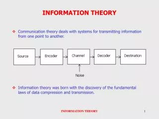
Information Theory • First developed by Shannon as a way of quantifying capacity of signal channels. • Entropy, relative entropy and mutual information capture intrinsic informational aspects of a signal • Today: • Information theory provides a domain-independent way to reason about structure in data • More information = interesting structure • Less information linkage = decoupling of structures
Tutorial Thesis Information theory provides a mathematical framework for the quantification of information content, linkage and loss. This framework can be used in the design of data management strategies that rely on probing the structure of information in data.
Tutorial Goals • Introduce information-theoretic concepts to VLDB audience • Give a ‘data-centric’ perspective on information theory • Connect these to applications in data management • Describe underlying computational primitives Illuminate when and how information theory might be of use in new areas of data management.
Outline Part 1 Introduction to Information Theory Application: Data Anonymization Application: Data Integration Part 2 Review of Information Theory Basics Application: Database Design Computing Information Theoretic Primitives Open Problems 7
X f(X) X p(X) X x1 4 x1 0.5 aggregate counts x1 x2 2 x2 0.25 normalize x3 1 x3 0.125 x3 x4 1 x4 0.125 x2 x4 Probability distribution Histogram x1 x1 Column of data x2 x1 Histograms And Discrete Distributions
X f(X) X p(X) X x1 4 x1 0.667 aggregate counts x1 x2 2 x2 0.2 x3 1 x3 0.067 x3 x4 1 x4 0.067 x2 x4 Probability distribution Histogram x1 x1 Column of data x2 x1 Histograms And Discrete Distributions reweight normalize
From Columns To Random Variables • We can think of a column of data as “represented” by a random variable: • X is a random variable • p(X) is the column of probabilities p(X = x1), p(X = x2), and so on • Also known (in unweighted case) as the empirical distribution induced by the column X. • Notation: • X (upper case) denotes a random variable (column) • x (lower case) denotes a value taken by X (field in a tuple) • p(x) is the probability p(X = x)
Joint Distributions Discrete distribution: probability p(X,Y,Z) p(Y) = ∑x p(X=x,Y) = ∑x ∑z p(X=x,Y,Z=z) 11 11
Let h(x) = log2 1/p(x) h(X) is column of h(x) values. H(X) = EX[h(x)] = SX p(x) log2 1/p(x) Two views of entropy It captures uncertainty in data: high entropy, more unpredictability It captures information content: higher entropy, more information. Entropy Of A Column H(X) = 1.75 < log |X| = 2
Examples • X uniform over [1, ..., 4]. H(X) = 2 • Y is 1 with probability 0.5, in [2,3,4] uniformly. • H(Y) = 0.5 log 2 + 0.5 log 6 ~= 1.8 < 2 • Y is more sharply defined, and so has less uncertainty. • Z uniform over [1, ..., 8]. H(Z) = 3 > 2 • Z spans a larger range, and captures more information X Y Z
Comparing Distributions • How do we measure difference between two distributions ? • Kullback-Leibler divergence: • dKL(p, q) = Ep[ h(q) – h(p) ] = Si pi log(pi/qi) Inference mechanism Prior belief Resulting belief
Comparing Distributions • Kullback-Leibler divergence: • dKL(p, q) = Ep[ h(q) – h(p) ] = Si pi log(pi/qi) • dKL(p, q) >= 0 • Captures extra information needed to capture p given q • Is asymmetric ! dKL(p, q) != dKL(q, p) • Is not a metric (does not satisfy triangle inequality) • There are other measures: • 2-distance, variational distance, f-divergences, …
Conditional Probability • Given a joint distribution on random variables X, Y, how much information about X can we glean from Y ? • Conditional probability: p(X|Y) • p(X = x1 | Y = y1) = p(X = x1, Y = y1)/p(Y = y1)
Conditional Entropy • Let h(x|y) = log2 1/p(x|y) • H(X|Y) = Ex,y[h(x|y)] = SxSy p(x,y) log2 1/p(x|y) • H(X|Y) = H(X,Y) – H(Y) • H(X|Y) = H(X,Y) – H(Y) = 2.25 – 1.5 = 0.75 • If X, Y are independent, H(X|Y) = H(X)
Mutual Information • Mutual information captures the difference between the joint distribution on X and Y, and the marginal distributions on X and Y. • Let i(x;y) = log p(x,y)/p(x)p(y) • I(X;Y) = Ex,y[I(X;Y)] = SxSy p(x,y) log p(x,y)/p(x)p(y)
Mutual Information: Strength of linkage • I(X;Y) = H(X) + H(Y) – H(X,Y) = H(X) – H(X|Y) = H(Y) – H(Y|X) • If X, Y are independent, then I(X;Y) = 0: • H(X,Y) = H(X) + H(Y), so I(X;Y) = H(X) + H(Y) – H(X,Y) = 0 • I(X;Y) <= max (H(X), H(Y)) • Suppose Y = f(X) (deterministically) • Then H(Y|X) = 0, and so I(X;Y) = H(Y) – H(Y|X) = H(Y) • Mutual information captures higher-order interactions: • Covariance captures “linear” interactions only • Two variables can be uncorrelated (covariance = 0) and have nonzero mutual information: • X R [-1,1], Y = X2. Cov(X,Y) = 0, I(X;Y) = H(X) > 0
Information-Theoretic Clustering • Clustering takes a collection of objects and groups them. • Given a distance function between objects • Choice of measure of complexity of clustering • Choice of measure of cost for a cluster • Usually, • Distance function is Euclidean distance • Number of clusters is measure of complexity • Cost measure for cluster is sum-of-squared-distance to center • Goal: minimize complexity and cost • Inherent tradeoff between two
X f(X) X p(X) X v1 4 v1 0.5 aggregate counts v1 v2 2 v2 0.25 normalize v3 1 v3 0.125 v3 v4 1 v4 0.125 v2 v4 Probability distribution Histogram v1 v1 Column of data v2 v1 Feature Representation Let V = {v1, v2, v3, v4} X is “explained” by distribution over V. “Feature vector” of X is [0.5, 0.25, 0.125, 0.125]
Feature Representation p(v2|X2) = 0.2 Feature vector
Information-Theoretic Clustering • Clustering takes a collection of objects and groups them. • Given a distance function between objects • Choice of measure of complexity of clustering • Choice of measure of cost for a cluster • In information-theoretic setting • What is the distance function ? • How do we measure complexity ? • What is a notion of cost/quality ? • Goal: minimize complexity and maximize quality • Inherent tradeoff between two
Measuring complexity of clustering • Take 1: complexity of a clustering = #clusters • standard model of complexity. • Doesn’t capture the fact that clusters have different sizes.
Measuring complexity of clustering • Take 2: Complexity of clustering = number of bits needed to describe it. • Writing down “k” needs log k bits. • In general, let cluster t T have |t| elements. • set p(t) = |t|/n • #bits to write down cluster sizes = H(T) = S pt log 1/pt H( ) < H( )
Information-theoretic Clustering (take I) • Given data X = x1, ..., xn explained by variable V, partition X into clusters (represented by T) such that H(T) is minimized and quality is maximized
Soft clusterings • In a “hard” clustering, each point is assigned to exactly one cluster. • Characteristic function • p(t|x) = 1 if x t, 0 if not. • Suppose we allow points to partially belong to clusters: • p(T|x) is a distribution. • p(t|x) is the “probability” of assigning x to t How do we describe the complexity of a clustering ?
Measuring complexity of clustering • Take 1: • p(t) = Sx p(x) p(t|x) • Compute H(T) as before. • Problem: H(T1) = H(T2) !!
Measuring complexity of clustering • By averaging the memberships, we’ve lost useful information. • Take II: Compute I(T;X) ! • Even better: If T is a hard clustering of X, then I(T;X) = H(T) I(T2;X) = 0.46 I(T1;X) = 0
Information-theoretic Clustering (take II) • Given data X = x1, ..., xn explained by variable V, partition X into clusters (represented by T) such that I(T,X) is minimized and quality is maximized
Measuring cost of a cluster Given objects Xt = {X1, X2, …, Xm} in cluster t, Cost(t) = (1/m)Si d(Xi, C) = Si p(Xi) dKL(p(V|Xi), C) where C = (1/m) Si p(V|Xi) = Sip(Xi) p(V|Xi) = p(V)
Mutual Information = Cost of Cluster Cost(t) = (1/m)Si d(Xi, C) = Si p(Xi) dKL(p(V|Xi), p(V)) Si p(Xi) KL( p(V|Xi), p(V)) = Si p(Xi) Sj p(vj|Xi) log p(vj|Xi)/p(vj) = Si,j p(Xi, vj) log p(vj, Xi)/p(vj)p(Xi) = I(Xt, V) !! Cost of a cluster = I(Xt,V)
Cost of a clustering • If we partition X into k clusters X1, ..., Xk Cost(clustering) = Si pi I(Xi, V) (pi = |Xi|/|X|)
Cost of a clustering • Each cluster center t can be “explained” in terms of V: • p(V|t) = Si p(Xi) p(V|Xi) • Suppose we treat each cluster center itself as a point:
Cost of a clustering • We can write down the “cost” of this “cluster” • Cost(T) = I(T;V) • Key result [BMDG05] : Cost(clustering) = I(X, V) – (T, V) Minimizing cost(clustering) => maximizing I(T, V)
Information-theoretic Clustering (take III) • Given data X = x1, ..., xn explained by variable V, partition X into clusters (represented by T) such that I(T;X) - bI(T;V) is maximized • This is the Information Bottleneck Method [TPB98] • Agglomerative techniques exist for the case of ‘hard’ clusterings • b is the tradeoff parameter between complexity and cost • I(T;X) and I(T;V) are in the same units.
Information Theory: Summary • We can represent data as discrete distributions (normalized histograms) • Entropy captures uncertainty or information content in a distribution • The Kullback-Leibler distance captures the difference between distributions • Mutual information and conditional entropy capture linkage between variables in a joint distribution • We can formulate information-theoretic clustering problems
Outline Part 1 Introduction to Information Theory Application: Data Anonymization Application: Data Integration Part 2 Review of Information Theory Basics Application: Database Design Computing Information Theoretic Primitives Open Problems
Data Anonymization Using Randomization Goal: publish anonymized microdata to enable accurate ad hoc analyses, but ensure privacy of individuals’ sensitive attributes Key ideas: Randomize numerical data: add noise from known distribution Reconstruct original data distribution using published noisy data Issues: How can the original data distribution be reconstructed? What kinds of randomization preserve privacy of individuals? 39 Information Theory for Data Management - Divesh & Suresh
Data Anonymization Using Randomization Many randomization strategies proposed [AS00, AA01, EGS03] Example randomization strategies: X in [0, 10] R = X + μ (mod 11), μ is uniform in {-1, 0, 1} R = X + μ (mod 11), μ is in {-1 (p = 0.25), 0 (p = 0.5), 1 (p = 0.25)} R = X (p = 0.6), R = μ, μ is uniform in [0, 10] (p = 0.4) Question: Which randomization strategy has higher privacy preservation? Quantify loss of privacy due to publication of randomized data 40 Information Theory for Data Management - Divesh & Suresh
Data Anonymization Using Randomization X in [0, 10], R1 = X + μ (mod 11), μ is uniform in {-1, 0, 1} 41 Information Theory for Data Management - Divesh & Suresh
Data Anonymization Using Randomization X in [0, 10], R1 = X + μ (mod 11), μ is uniform in {-1, 0, 1} → 42 Information Theory for Data Management - Divesh & Suresh
Data Anonymization Using Randomization X in [0, 10], R1 = X + μ (mod 11), μ is uniform in {-1, 0, 1} → 43 Information Theory for Data Management - Divesh & Suresh
Reconstruction of Original Data Distribution X in [0, 10], R1 = X + μ (mod 11), μ is uniform in {-1, 0, 1} Reconstruct distribution of X using knowledge of R1 and μ EM algorithm converges to MLE of original distribution [AA01] → → 44 Information Theory for Data Management - Divesh & Suresh
Analysis of Privacy [AS00] X in [0, 10], R1 = X + μ (mod 11), μ is uniform in {-1, 0, 1} If X is uniform in [0, 10], privacy determined by range of μ → → 45 Information Theory for Data Management - Divesh & Suresh
Analysis of Privacy [AA01] X in [0, 10], R1 = X + μ (mod 11), μ is uniform in {-1, 0, 1} If X is uniform in [0, 1] [5, 6], privacy smaller than range of μ → → 46 Information Theory for Data Management - Divesh & Suresh
Analysis of Privacy [AA01] X in [0, 10], R1 = X + μ (mod 11), μ is uniform in {-1, 0, 1} If X is uniform in [0, 1] [5, 6], privacy smaller than range of μ In some cases, sensitive value revealed → → 47 Information Theory for Data Management - Divesh & Suresh
Quantify Loss of Privacy [AA01] Goal: quantify loss of privacy based on mutual information I(X;R) Smaller H(X|R) more loss of privacy in X by knowledge of R Larger I(X;R) more loss of privacy in X by knowledge of R I(X;R) = H(X) – H(X|R) I(X;R)used to capture correlation between X and R p(X) is the prior knowledge of sensitive attribute X p(X, R) is the joint distribution of X and R 48 Information Theory for Data Management - Divesh & Suresh
Quantify Loss of Privacy [AA01] Goal: quantify loss of privacy based on mutual information I(X;R) X is uniform in [5, 6], R1 = X + μ (mod 11), μ is uniform in {-1, 0, 1} 49 Information Theory for Data Management - Divesh & Suresh
Quantify Loss of Privacy [AA01] Goal: quantify loss of privacy based on mutual information I(X;R) X is uniform in [5, 6], R1 = X + μ (mod 11), μ is uniform in {-1, 0, 1} 50 Information Theory for Data Management - Divesh & Suresh