Download
1 / 22
220 likes | 353 Views
Strategies for improving seasonal prediction . Tim Stockdale, Franco Molteni , Magdalena Balmaseda , Kristian Mogensen and Laura Ferranti. Outline. The seasonal prediction problem is tough The need for accuracy : DJF 2011/12 Sampling limitations Forecast system improvements

E N D
Strategies for improving seasonal prediction Tim Stockdale, Franco Molteni, Magdalena Balmaseda, KristianMogensen and Laura Ferranti
Outline • The seasonal prediction problem is tough • The need for accuracy: DJF 2011/12 • Sampling limitations • Forecast system improvements • Example of ECMWF System 4 • Benefits can be demonstrated, but challenges remain • Benefits of multi-model • Conclusions
MSLP DJF 2011/12, ECMWF S3: Ensemble mean Prob MSLP > median
Sampling limitations • Re-forecasts have small number of events • Each forecast givesa pdf – obs could be anywhere in that pdf • For low or intermittent signal areas, 30 years is a very small sample! • Re-forecasts are (usually) small ensembles • Forecast pdfs are not that well sampled, especially in re-forecasts • Easy to end up calculating scores by correlating “mostly noise” with “mostly noise” …. • One practical benefit of multi-model – spreads the cost of producing large hindcast ensembles (eg 100 members, 30 years, 12 start dates, 7 months = 21,000 years of model integration)
An improved forecast system: • ECMWF System 4 • Replaces System 3, operational since March 2007 • Many changes, lots of testing, large re-forecast set now complete • Major model changes • NEMO ocean model replaces HOPE. Similar resolution, but better mixed layer physics. • New IFS cycle 36r4 (circa 5 years progress) • T255 horizontal resolution (cf T159) • L91, and enhanced stratospheric physics (cf L62) • Stochastic physics: SPPT3 and stochastic backscatter instead of old SPPT: SPPT3 represents model uncertainty – big spread in ENSO forecasts • Ice sampled from preceding five years instead of fixed climatology
S4 initial conditions • Major initial condition changes • NEMOVAR ocean analysis/re-analysis. New 3D-VAR system, incorporating all major elements of previous system, but many aspects of re-analyses are improved. • Land surface initial conditions: offline run of HTESSEL, with GPCP-corrected ERA interim forcing (re-forecasts); operational analyses (forecasts). • ERA Interim initial conditions for atmosphere to end 2010, then operations • Stratospheric ozone from climatology of selected ERA interim years (direct use of ozone analysis problematic). • Volcanic aerosol input as NH/TROPICS/SH zonal mean values at start of each integration
Benefits of an improved system • Much better mean state • Mostly much better, but one important thing is worse • Progress is real, but not monotonic and not easy (experience of many modelling groups over the last 20 years) • Better ENSO forecasts • Much better in NINO3, bit better in NINO34, bit worse in NINO4 • Amplitude of ENSO too strong, mean state error problems • Better atmospheric forecasts • Very strong consistent improvements in tropics, and strong improvements in NH scores also (but not all months, eg NH winter Z500 noisy) • Strong improvements both in ACC and in reliability scores • Big improvements, but not a “perfect” system yet!
Mean state errors S4 S3 T850 U50
Mean state 925hPa winds S4 S3 Overall biases are reduced, but wind bias in equatorial West Pacific is a problem
Tropospheric scores: ACC statistics (30y) Statistic=z-transform spatial mean of ACC of 3 month forecast, 1981-2010 Assessed for each of 12 possible start months, and scores aggregated “NH” is poleward of 30N, “Tropics” is 30N-30S
(Some) Future ECMWF developments • Better atmosphere/ocean models • Reduction of equatorial wind bias, plus other improvements. Evidence suggests higher resolution atmosphere will play a role. • Tropospheric aerosol variations • Higher resolution ocean • Land surface • Full offline re-analysis of land surface initial conditions, esp snow • Fully consistent real-time initialization • Improvements: vegetation response, hydrology • Stratosphere • Spectrally resolved UV radiation, to allow proper impact of solar variability • Increased vertical resolution, to allow better QBO dynamics • Better (post eruption) volcanic aerosol specification, better ozone • Sea-ice • Actually having a model ….
Multi-model approach • Operational multi-model system at ECMWF • Called EUROSIP, initially ECMWF/Met Office/Meteo-France • NCEP have now joined • Others intending to join • Multi-model likes high quality models • Automatically benefit • May be some issues if there is a mix of excellent models and poor ones • Ideally like long re-forecast set and skill estimates for each model • Past research has shown multi-model hard to beat
0.170 0.959 0.211 0.222 0.994 0.227 Hagedorn et al. (2005) DEMETER: impact of ensemble size 1-month lead, start date May, 1987 - 1999 BSS Rel-Sc Res-Sc Reliability diagrams (T2m > 0) 1-month lead, start date May, 1987 - 1999 multi-model [54 members] single-model [54 members]
Cf benefit from model improvement 0.132 0.920 0.212 0.217 0.963 0.254 S3 S4
Conclusions • Producing good forecasts is hard • Models need to include relevant processes to a high accuracy • Models need to be complete, including all main sources of variability • Verifying forecasts is hard • Large ensemble sizes needed to properly characterize pdfs • Limited number of events to look at modest shifts in pdfs • Multi-model forecasts are very useful • They always give a sanity check • They can be combined to give more reliable and usually better forecasts • Keep up the work on the forecast systems … • To produce most informative forecasts possible • Need to aim at being intrinsically reliable