Download
1 / 1
10 likes | 85 Views
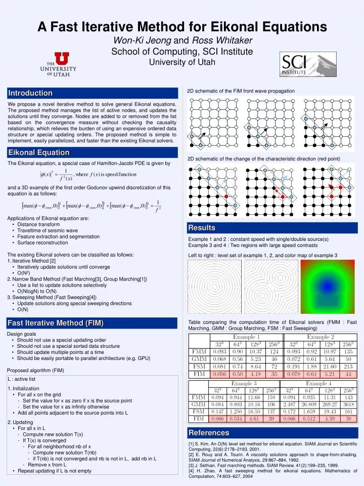
2D schematic of the change of the characteristic direction (red point). Introduction.

E N D
2D schematic of the change of the characteristic direction (red point) Introduction We propose a novel iterative method to solve general Eikonal equations. The proposed method manages the list of active nodes, and updates the solutions until they converge. Nodes are added to or removed from the list based on the convergence measure without checking the causality relationship, which relieves the burden of using an expensive ordered data structure or special updating orders. The proposed method is simple to implement, easily parallelized, and faster than the existing Eikonal solvers. Eikonal Equation The Eikonal equation, a special case of Hamilton-Jacobi PDE is given by and a 3D example of the first order Godunov upwind discretization of this equation is as follows: 2D schematic of the FIM front wave propagation • Applications of Eikonal equation are: • Distance transform • Traveltime of seismic wave • Feature extraction and segmentation • Surface reconstruction • The existing Eikonal solvers can be classified as follows: • Iterative Method [2] • Iteratively update solutions until converge • O(N2) • Narrow Band Method (Fast Marching[3], Group Marching[1]) • Use a list to update solutions selectively • O(NlogN) to O(N) • Sweeping Method (Fast Sweeping[4]) • Update solutions along special sweeping directions • O(N) Results References Example 1 and 2 : constant speed with single/double source(s) Example 3 and 4 : Two regions with large speed contrasts Left to right : level set of example 1, 2, and color map of example 3 Table comparing the computation time of Eikonal solvers (FMM : Fast Marching, GMM : Group Marching, FSM : Fast Sweeping) [1] S. Kim. An O(N) level set method for eikonal equation. SIAM Journal on Scientific Computing, 22(6):2178–2193, 2001. [2] E. Rouy and A. Tourin. A viscosity solutions approach to shape-from-shading. SIAM Journal of Numerical Analysis, 29:867–884, 1992. [3] J. Sethian. Fast marching methods. SIAM Review, 41(2):199–235, 1999. [4] H. Zhao. A fast sweeping method for eikonal equations. Mathematics of Computation, 74:603–627, 2004 Fast Iterative Method (FIM) • Design goals • Should not use a special updating order • Should not use a special sorted data structure • Should update multiple points at a time • Should be easily portable to parallel architecture (e.g. GPU) • Proposed algorithm (FIM) • L : active list • Initialization • For all x on the grid • Set the value for x as zero if x is the source point • Set the value for x as infinity otherwise • Add all points adjacent to the source points into L • Updating • For all x in L • Compute new solution T(x) • If T(x) is converged • For all neighborhood nb of x • Compute new solution T(nb) • if T(nb) is not converged and nb is not in L, add nb in L • Remove x from L • Repeat updating if L is not empty A Fast Iterative Method for Eikonal Equations Won-Ki Jeong and Ross Whitaker School of Computing, SCI Institute University of Utah