Download
1 / 8
80 likes | 382 Views
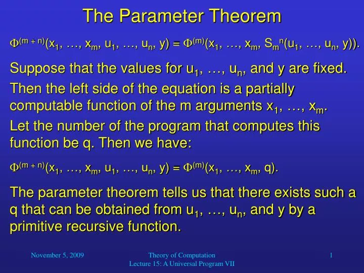
The Parameter Theorem. (m + n) (x 1 , …, x m , u 1 , …, u n , y) = (m) (x 1 , …, x m , S m n (u 1 , …, u n , y)). Suppose that the values for u 1 , …, u n , and y are fixed. Then the left side of the equation is a partially computable function of the m arguments x 1 , …, x m .

E N D
The Parameter Theorem (m + n)(x1, …, xm, u1, …, un, y) = (m)(x1, …, xm, Smn(u1, …, un, y)). Suppose that the values for u1, …, un, and y are fixed. Then the left side of the equation is a partially computable function of the m arguments x1, …, xm. Let the number of the program that computes this function be q. Then we have: (m + n)(x1, …, xm, u1, …, un, y) = (m)(x1, …, xm, q). The parameter theorem tells us that there exists such a q that can be obtained from u1, …, un, and y by a primitive recursive function. Theory of Computation Lecture 15: A Universal Program VII
The Parameter Theorem Let us take a look at the case n = 1: (m + 1)(x1, …, xm, u, y) = (m)(x1, …, xm, Sm1(u, y)). Here, Sm1(u, y) is the number of a program that receives inputs x1, …, xm and computes the same value as program number y does on inputs x1, …, xm, and u. We can easily obtain Sm1(u, y) by writing the instruction Xm+1 u and then appending the program with number y. This works similarly for any given n, which can be proven by mathematical induction (see page 86 in the textbook). Theory of Computation Lecture 15: A Universal Program VII
Diagonalization and Reducibility We will now look at two techniques for proving that a set is not recursive or not even r.e. These techniques are called diagonalization and reducibility. The idea behind diagonalization is to conduct a proof by contradiction. First, we make the assumption that a certain set A can be enumerated in a suitable fashion. Second, we show that, with the help of the enumeration, we can define an object b with b A. Theory of Computation Lecture 15: A Universal Program VII
Diagonalization and Reducibility For example, we proved Theorem 2.1 using a diagonalization argument to show that HALT(x, y) or {(x, y) N2 | HALT(x, y)} is not computable. Here, the set A is the class of unary partially computable functions. Assertion 1 (A can be enumerated) follows from the fact that L programs can be enumerated. For each n, let Pn be the program with number n. Then all unary partially computable functions are in the following list: (1)P0, (1)P1, (1)P2, … Theory of Computation Lecture 15: A Universal Program VII
Diagonalization and Reducibility We first assumed that HALT(x, y) were computable and performed a proof by contradiction. Then we wrote a program P that computes (1)P which involved the (assumedly computable) predicate HALT(x, y). Finally, we showed that (1)P does not appear in the list (1)P0, (1)P1, (1)P2, … From this contradiction we concluded that HALT(x, y) cannot be computable. Theory of Computation Lecture 15: A Universal Program VII
Diagonalization and Reducibility The idea was to write P such that for every x, (1)P(x) if and only if (1)Px(x). In other words, HALT(x, #(P )) HALT(x, x) This means that (1)P(x) differs from each function (1)P0, (1)P1, (1)P2, … on at least one input value. (1)P cannot be (1)Pn, because (1)P (n) if and only if (1)Pn (n). Theory of Computation Lecture 15: A Universal Program VII
Diagonalization and Reducibility So (1)P does not appear in the list (1)P0, (1)P1, (1)P2, …, which satisfies Assertion 2 (there is a b A). By this contradiction we can conclude that HALT(x, y) is not computable. The term diagonalization is derived from the visualization of this proof technique. Theory of Computation Lecture 15: A Universal Program VII
Diagonalization (1)P0 (0) (1)P0 (1) (1)P0 (2) … (1)P1 (0) (1)P1 (1) (1)P1 (2) … (1)P2 (0) (1)P2 (1) (1)P2 (2) … … … … … The elements on the diagonal make it impossible for (1)P to be any of the (1)Pn. Theory of Computation Lecture 15: A Universal Program VII