Download
1 / 167
1.68k likes | 1.87k Views
METAHEURISTICS Neighborhood (Local) Search Techniques. Jacques A. Ferland Department of Informatique and Recherche Opérationnelle Université de Montréal ferland@iro.umontreal.ca. Introduction. Introduction to some basic methods My vision relying on my experience Not an exaustive survey

E N D
METAHEURISTICSNeighborhood (Local) Search Techniques Jacques A. Ferland Department of Informatique and Recherche Opérationnelle Université de Montréal ferland@iro.umontreal.ca
Introduction • Introduction to some basic methods • My vision relying on my experience • Not an exaustive survey • Most of the time ad hoc adaptations of basic methods are used to deal with specific applications
Advantages of using metaheuristic • Intuitive and easy to understand • With regards to enduser of a real world application: - Easy to explain - Connection with the manual approach of enduser - Enduser sees easily the added features to improve the results - Allow to analyze more deeply and more scenarios • Allow dealing with larger size problems having higher degree of complexity • Generate rapidly very good solutions
Disadvantages of using metaheuristic • Quick and dirty methods • Optimality not guaranted in general • Few convergence results for special cases
Summary • Heuristic Constructive techniques: Greedy GRASP (Greedy Randomized Adaptive Search Procedure) • Neighborhood (Local) Search Techniques: Descent Tabu Search Simulated Annealing Threshold Accepting • Improving strategies Intensification Diversification Variable Neighborhood Search (VNS) Exchange Procedure
Problem used to illustrate • General problem min f(x) x є X • Assignment type problem: Assignment of resources j to activities i min f(x) Subject to ∑1≤ j≤ mxij = 1 1≤ i ≤ n xij = 0 or 1 1≤ i ≤ n, 1≤ j ≤ m
Problem Formulation • Assignment type problem min f(x) Subject to ∑1≤ j≤ m xij = 1 1≤ i ≤ n xij = 0 or 1 1≤ i ≤ n, 1≤j ≤ m • Graph coloring problem : Graph G = (V,E). V = { i : 1≤ i ≤ n} ; E = {(i, l): (i, l)edge of G}. Set of colors {j :1≤ j ≤ m} min ∑ 1≤ j≤ m∑ (i, l) є E xij xlj Subject to ∑1≤ j≤ m xij = 1 1≤ i ≤ n xij = 0 or 1 1≤ i ≤ n, 1≤ j ≤ m
Graph coloring example • Graph coloring problem : Graph G = (V,E). V = { i : 1≤ i ≤ n} ; E = {(i, l): (i, l)edge of G}. Set of colors {j :1≤ j ≤ m} min f(x) = ∑ 1≤ j≤ m∑ (i, l) є E xij xlj Subject to ∑1≤ j≤ m xij = 1 1≤ i ≤ n xij = 0 or 1 1≤ i ≤ n, 1≤ j ≤ m • To simplify notation, denote or encode a solution x as follows: x =>[j(1), j(2),…, j(i), …, j(n)] where for each vertex i, xij(i) = 1 xij = 0 for all other j
Heuristic Constructive Techniques • Values of the variables are determined sequentially: at each iteration, a variable is selected, and its value is determined • The value of each variable is never modifided once it is determined • Techniques often used to generate initial solutions for iterative procedures
Next variable to be fixed and its value are selected to optimize the objective function given the values of the variables already fixed Graph coloring problem: Vertices are ordered in decreasing order of their degree Vertices selected in that order For each vertex, select a color in order to reduce the number of pairs of adjacent vertices already colored with the same color Greedy method
Graph coloring example • Graph with 5 vertices • 2 colors available: red blue
Graph coloring example • Vertices in decreasing order of degree • Vertex degree color 2 3 1 2 3 2 4 2 5 1
Graph coloring example • Vertices in decreasing order of degree • Vertex degree color 2 3 1 2 3 2 4 2 5 1 • Vertex 2 color number of adj. vert. same color red 0 blue 0 <=
Graph coloring example • Vertices in decreasing order of degree • Vertex degree color 2 3 blue 1 2 3 2 4 2 5 1 • Vertex 2 color number of adj. vert. same color red 0 blue 0 <=
Graph coloring example • Vertices in decreasing order of degree • Vertex degree color 2 3 blue 1 2 3 2 4 2 5 1
Graph coloring example • Vertices in decreasing order of degree • Vertex degree color 2 3 blue 1 2 3 2 4 2 5 1 • Vertex 1 color number of adj. vert. same color red 0 <= blue 1
Graph coloring example • Vertices in decreasing order of degree • Vertex degree color 2 3 blue 1 2 red 3 2 4 2 5 1 • Vertex 1 color number of adj. vert. same color red 0 <= blue 1
Graph coloring example • Vertices in decreasing order of degree • Vertex degree color 2 3 blue 1 2 red 3 2 4 2 5 1
Graph coloring example • Vertices in decreasing order of degree • Vertex degree color 2 3 blue 1 2 red 3 2 4 2 5 1 • Vertex 3 color number of adj. vert. same color red 1 <= blue 1
Graph coloring example • Vertices in decreasing order of degree • Vertex degree color 2 3 blue 1 2 red 3 2 red 4 2 5 1 • Vertex 3 color number of adj. vert. same color red 1 <= blue 1
Graph coloring example • Vertices in decreasing order of degree • Vertex degree color 2 3 blue 1 2 red 3 2 red 4 2 5 1
Graph coloring example • Vertices in decreasing order of degree • Vertex degree color 2 3 blue 1 2 red 3 2 red 4 2 5 1 • Vertex 4 color number of adj. vert. same color red 0 <= blue 1
Graph coloring example • Vertices in decreasing order of degree • Vertex degree color 2 3 blue 1 2 red 3 2 red 4 2 red 5 1 • Vertex 4 color number of adj. vert. same color red 0 <= blue 1
Graph coloring example • Vertices in decreasing order of degree • Vertex degree color 2 3 blue 1 2 red 3 2 red 4 2 red 5 1
Graph coloring example • Vertices in decreasing order of degree • Vertex degree color 2 3 blue 1 2 red 3 2 red 4 2 red 5 1 • Vertex 5 color number of adj. vert. same color red 1 blue 0 <=
Graph coloring example • Vertices in decreasing order of degree • Vertex degree color 2 3 blue 1 2 red 3 2 red 4 2 red 5 1 blue • Vertex 5 color number of adj. vert. same color red 1 blue 0 <=
GRASPGreedy Randomized Adaptive Search Procedure • Next variable to be fixed is selected randomly among those inducing the smallest increase. • Referring to the general problem, i) let J’ = { j : xjis not fixed yet} and δjbe the increase induces by the best value thatxj can take ( j є J’ ) ii) Denote δ* = min j є J’{ δj } and αє [0, 1] . iii) Select randomly j’є {j є J’ : δj≤ ( 1 / α) δ* } and fix the value of xj’
Graph coloring example • Graph with 5 vertices • 2 colors available: red blue • α = 0.5
Graph coloring example Vertex j best color δj color 1 any 0 2 any 0 3 any 0 4 any 0 5 any 0
Graph coloring example Vertex j best color δj color 1 any 0 2 any 0 3 any 0 4 any 0 5 any 0 J’ = {1, 2, 3, 4, 5} δ* = 0 α = 0.5 {j є J’ : δj≤ ( 1 / α) δ* }= {1, 2, 3, 4, 5} • Select randomly vertex 3 color blue
Graph coloring example Vertex j best color δj color 1 any 0 2 any 0 3 any 0 blue 4 any 0 5 any 0 J’ = {1, 2, 3, 4, 5} δ* = 0 α = 0.5 {j є J’ : δj≤ ( 1 / α) δ* }= {1, 2, 3, 4, 5} • Select randomly vertex 3 color blue
Graph coloring example Vertex j best color δj color 1 red 0 2 red 0 3 blue 4 any 0 5 any 0
Graph coloring example Vertex j best color δj color 1 red 0 2 red 0 3 blue 4 any 0 5 any 0 J’ = {1, 2, 4, 5} δ* = 0 α = 0.5 {j є J’ : δj≤ ( 1 / α) δ* }= {1, 2, 4, 5} • Select randomly vertex 4 color red
Graph coloring example Vertex j best color δj color 1 red 0 2 red 0 3 blue 4 any 0 red 5 any 0 J’ = {1, 2, 4, 5} δ* = 0 α = 0.5 {j є J’ : δj≤ ( 1 / α) δ* }= {1, 2, 4, 5} • Select randomly vertex 4 color red
Graph coloring example Vertex j best color δj color 1 red 0 2 any 1 3 blue 4 red 5 blue 0
Graph coloring example Vertex j best color δj color 1 red 0 2 any 1 3 blue 4 red 5 blue 0 J’ = {1, 2, 5} δ* = 0 α = 0.5 {j є J’ : δj≤ ( 1 / α) δ* }= {1, 5} • Select randomly vertex 5 color blue
Graph coloring example Vertex j best color δj color 1 red 0 2 any 1 3 blue 4 red 5 blue 0 blue J’ = {1, 2, 5} δ* = 0 α = 0.5 {j є J’ : δj≤ ( 1 / α) δ* }= {1, 5} • Select randomly vertex 5 color blue
Graph coloring example Vertex j best color δj color 1 red 0 2 any 1 3 blue 4 red 5 blue
Graph coloring example Vertex j best color δj color 1 red 0 2 any 1 3 blue 4 red 5 blue J’ = {1, 2} δ* = 0 α = 0.5 {j є J’ : δj≤ ( 1 / α) δ* }= {1} • Select vertex 1 color red
Graph coloring example Vertex j best color δj color 1 red 0 red 2 any 1 3 blue 4 red 5 blue J’ = {1, 2} δ* = 0 α = 0.5 {j є J’ : δj≤ ( 1 / α) δ* }= {1} • Select vertex 1 color red
Graph coloring example Vertex j best color δj color 1 red 2 blue 1 3 blue 4 red 5 blue
Graph coloring example Vertex j best color δj color 1 red 2 blue 1 3 blue 4 red 5 blue J’ = {2} δ* = 1 α = 0.5 {j є J’ : δj≤ ( 1 / α) δ* }= {2} • Select vertex 2 color blue
Graph coloring example Vertex j best color δj color 1 red 2 blue 1 blue 3 blue 4 red 5 blue J’ = {2} δ* = 1 α = 0.5 {j є J’ : δj≤ ( 1 / α) δ* }= {2} • Select vertex 2 color blue
Graph coloring example Vertex j best color δj color 1 red 2 blue 3 blue 4 red 5 blue J’ = Φ
Neighborhood (Local) Search Techniques (NST) • A Neighborhood (Local) Search Technique (NST) is an iterative procedure starting with an initial feasible solution x0. • At each iteration: - we move from the current solution x є X to a new one x'є X in its neighborhood N(x) - x' becomes the current solution for the next iteration - we update the best solution x* found so far. • The procedure continues until some stopping criterion is satisfied
Neighborhood Neighborhood N(x): The neighborhood N(x)varies with the problem, but its elements are always generated by slightly modifying x. If we denote M the set of modifications (or moves) to generate neighboring solutions, then N(x) = {x' : x' = x mo , mo M }
Neighborhood for assigment type problem • For theassignment type problem: Let x be as follows: for each 1≤ i ≤ n, xij(i) = 1 xij = 0 for all other j Each solutionx'єN(x)is obtained byselecting an activity i and modifying its resource from j(i)tosome other p (i. e., the modification can be denoted mo = [i, p] ): x'ij(i) = 0 x'ip = 1 x'ij = xij for all other i, j The elements of the neighborhood N(x)are generated by slightly modifying x: N(x) = {x' : x' = x mo , mo M }
Neighborhood (Local) Search Techniques (NST) • Descent method • Tabu Search • Simulated Annealing • Threshold Accepting • Introduce these methods using pseudo-codes
Descent Method (D) • At each iteration, a best solution x' є N(x)is selected as the current solution for the next iteration. • Stopping criterion: f(x') ≥ f(x) i.e., the current solution cannot be improved or a first local minimum is reached.