Download
1 / 47
490 likes | 805 Views
Particle Physics 2. Prof. Glenn Patrick . U23525, Particle Physics, Year 3 University of Portsmouth, 2013 - 2014. Last Lecture. Particle Physics 1 Course Outline Preliminaries - Assessment Preliminaries - Books Preliminaries - Course Material

E N D
Particle Physics 2 Prof. Glenn Patrick U23525, Particle Physics, Year 3 University of Portsmouth, 2013 - 2014
Last Lecture Particle Physics 1 Course Outline Preliminaries - Assessment Preliminaries - Books Preliminaries - Course Material Particle Physics, Cosmology & Particle Astrophysics Natural Units Rationalised Heaviside-Lorentz EM Units Special Relativity and Lorentz Invariance Mandelstam Variables (s, t and u) Crossing Symmetry and s, t & u Channels Spin and Spin Statistics Theorem – Fermions and Bosons Addition of Angular Momentum Non-Relativistic Quantum Mechanics (Schrödinger Equation) Relativistic Quantum Mechanics (Klein-Gordon Equation) Feynman-Stückelberg Interpretation of Negative Energy States
Today’s Plan Particle Physics 2 Dirac Equation Dirac Interpretation of Negative States Stückelberg & Feynman Interpretations Discovery: Positron & e+e- Pair Production Decays – Lifetimes Scattering – Cross-sections Feynman Diagrams Quantum Electrodynamics (QED) Higher Order Diagrams LEP example Running Coupling Constant ( QED Renormalisation Electron/Positron Annihilation & precision LEP electroweak example
Correction - Assessment 40 hours of lectures across two teaching blocks plus 8 hours of tutorial classes. The main aim is to improve your understanding of fundamental physics. However, we cannot forget the small matter of your degree…. Final written examination (2 hours) – 80% Coursework questions and problems – 20% Not 3 hours as I said last week. • Main thing is that you enjoy the course. • We will try and focus on understanding the underlying concepts. • Extra material/maths shown mainly to aid understanding. • Guidance will be given over essential knowledge needed for exam.
Corrections - Timetable • There is NO lecture this afternoon at 15:00 – 17:00. The timetable was wrong. • There are also 2 extra weeks added in March to the end of teaching block 2 (weeks 34 and 35).
Moodle Site Slides - pptx Slides - pdf
2013 Nobel Prize – Particle Physics The Nobel Prize in Physics 2013 was awarded jointly to François Englert and Peter W. Higgs "for the theoretical discovery of a mechanism that contributes to our understanding of the origin of mass of subatomic particles, and which recently was confirmed through the discovery of the predicted fundamental particle, by the ATLAS and CMS experiments at CERN's Large Hadron Collider”.
Dirac Equation • The Klein Gordon equation was believed to be sick, but today we now understand it was telling us something about antiparticles. • To try to solve the problem of –ve energy solutions, Dirac: • Wanted an equation first order in . • Started by assuming a Hamiltonian, which is local and linear in p and of the form: To also make the equation relativistically covariant, it has to be linear in : Solutions of this equation were also required to be solutions of the Klein Gordon equation. Only true if: Coefficients do not commute so they cannot be numbers – require 4 matrices.
Dirac Equation In two dimensions, a natural set of matrices would be the Pauli spin matrices (from atomic physics for electron spin): but there is no suitable fourth anti-commuting matrix for β. Convenient choice is to instead use the Dirac-Pauli representation: 2 x 2 identity matrix These can be abbreviated as: (each element is a 2 x 2 matrix) Block matrix (2 x 2)
Dirac Equation Now that and are matrices, the equation makes no sense unless the wave function is itself a matrix with four rows and one column. This is the Dirac Spinor: (a four component wavefunction) Plane wave solutions take the form: where ) is also a four-component spinor satisfying the eigenvalue equation: There are four solutions: two with positive energy E = +Ep corresponding to the two possible spin states of a spin particle and two corresponding negative energy solutions with E = - Ep. Electron spin is therefore included in a natural way (rather than the previous ad-hoc attempts). All solutions also have positive probability density.
Dirac Interpretation • Dirac interpreted the negative energy solutions by: • Postulating the existence of a “sea” of negative energy states, which are almost always filled – each with two electrons (spin “up” and spin “down”): • When an electron is added to the vacuum, it is confined to the positive energy region since all negative energy states are occupied (Pauli exclusion principle). • When energy is supplied to promote a negative energy electron to a positive energy level, an electron-hole pair is created. The hole is seen as a charge +e and E > 0 state. A false start when Dirac identified negative energy electrons as protons. Eventually, persuaded by arguments of Weyl & Oppenheimer that +ve particle had to have the same mass as the electron.
Dirac Interpretation Photon with excites electron from –ve energy state. Leaves hole in vacuum corresponding to a state with more energy (less negative energy) and a positive charge wrt the vacuum. Sea • Problems with this picture. • Bosons have no exclusion principle, so this picture does not work for them. • It implies the Universe has infinite negative energy! • Nonetheless, in 1931 Dirac postulated the existence of the positron as the electron’s antiparticle. • It was discovered 1 year later.
Positron - First Antiparticle Discovered! e+ e- Positron = the anti-electron 6 mm lead plate e+ Discovered in 1932 by Carl Anderson photographing cosmic ray tracks in a cloud chamber.
Pair Production In 1933, Blackett & Occhialini observed pair production in a triggered cloud chamber and confirmed that Anderson’s particle was indeed Dirac’s positron.
Stückelberg Interpretation As early as 1941, Stückelberg cultivated the view that positrons may be understood as electrons running backward in time. E.C.G. Stueckelberg, Helvetica PhysicaActa, 14 (1941), 588-594
Feynman Interpretation “The problem of the behavior of positrons and electrons in given external potentials, neglecting their mutual interaction, is analyzed by replacing the theory of holes by a reinterpretation of the solutions of the Dirac equation…..”. …In this solution, the “negative energy states” appear in a form which may be pictured (as by Stückelberg) in space-time as waves traveling away from the external potential backwards in time. Experimentally, such a wave corresponds to a positron approaching the potential and annihilating the electron…. July 1962
Feynman Interpretation Waves can proceed backward in time Virtual pair production. Positron goes forward in time (4 to 3) to be annihilated and electron backwards (3 to 4)
One electron in the entire Universe? It was Feynman’s PhD supervisor, John Wheeler, who suggested that there may be only a single electron in the universe, propagating through space and time! • This obviously has a few problems! For example: • You would expect equal number of electrons and positrons and yet we observe extremely few positrons. • How do we account for the fact that electrons can be created/destroyed in weak interactions. • This poor single electron would have had to traverse huge distances and be very ancient. Nonetheless, Feynman kept the idea that positrons could simply be represented as electrons going from the future to the past. World-line of single electron
Reminder: this is Applied Physics! This quantum theory is all very well, but what can we physically measure? Applied Physicist Quantum Theorist
Decays - Lifetimes • In the case of particle decays, the most interesting physical quantity is the lifetime of the particle. • Measured in the rest frame of the particle. We can define the decay rate, , as the probability per unit time the particle will decay. Similar to your Year 2 nuclear physics Mean Lifetime (natural units) • Most particles decay by several different routes. The total • decay rate is then the sum of the individual decay rates: • The lifetime of the particle is then: • The different final states are known as decay modes. • The branching ratio for i’th decay mode is:
Meson Example Particle Data Group: http://pdg.lbl.gov/
Scattering - Cross-Section na = no. of beam particles va = velocity of beam particles nb = no. target particles/area Incident flux F=nava dN = no. scattered particles in solid angle dΩ Luminosity L = flux x no. targets (cm-2s-1) Differential cross-section Total cross-section Cross-section quantifies rate of reaction. Depends on underlying physics. Measured in barns. 1 b = 10-24 cm-2
Feynman Diagrams “Like the silicon chip of more recent years, the Feynman diagram was bringing computation to the masses”. Julian Schwinger
Feynman Diagrams – The Problem Consider the calculation of the cross-section of one of the simplest QED processes. In the Centre of Mass frame: where are momenta = QM amplitude for process. Bad News! Even for this simple process the exact expression is not known. Best that can be done is to obtain a formal expression for as a perturbation series in the strength of the EM interaction & evaluate the first few terms. Feynman invented a beautiful way to organise, visualise and thereby calculate the perturbation series.
Quantum Field Theory - Basics • In Quantum Field Theory, the scattering and decay of particles is described in terms of transition amplitudes. • For a transition process , the transition amplitude is written as , where S is an operator known as the Scattering Matrix or S-Matrix. • Exact calculations of are not possible, but it is possible to use perturbation theory which allow approximate calculations of the transition amplitude. • A bit like a binomial/Taylor series expansion: • e.g. and then keeping the first 2 terms in the expansion (for small values of x). • Feynman diagrams are a technique to solve quantum field theory by calculating the amplitude for a state with specified incoming and outgoing particles.
Feynman Diagrams - Basics Annihilation Diagram External legs represent amplitudes of initial & final state particles. boson (wavy line) Final State Initial State vertex vertex Internal lines (propagators) represent amplitude of exchanged particle. Exchange Diagram fermion (solid line) CONVENTION fermion gluons Virtual Particle anti-fermion H bosons photons, W, Z bosons • Time runs from left to right. • Particles point in +ve time direction. • Anti-particles point in –ve time direction. • Charge, energy, momentum, angular momentum, baryon no. & lepton no. conserved at interaction vertices. Quark flavour for strong & EM interactions.
Feynman Diagrams - Calculation • Perturbation theory. Expand and keep the most important terms for calculations. • Associate each vertex with the square root of the appropriate coupling constant, i.e. . • When the amplitude is squared to yield a cross-section there will be a factor , where n is the number of vertices (known as the “order” of the diagram). Second order Lowest order For QED: Add the amplitudes from all possible diagrams to get the total amplitude, M, for a process transition probability. Fermi’s Golden Rule “Just”kinematics Contains the fundamentalphysics
Phase Space Introduced by Willard Gibbs in 1901. Defines the space in which all possible states of a system are represented, with each possible state of the system corresponding to one unique point in the phase space. Example: 3 Body Decay Phase space illustrated by this 2-D plot of a three-body decay (a so-called “Dalitz plot”). The contour line shows the boundary of what is kinematically possible - i.e. the edge of phase space. Contour showing limit of kinematically available phase space. Crystal Barrel Experiment
Quantum Electrodynamics (QED) Early relativistic quantum theories had to be rethought after the discovery of the Lamb Shift in hydrogen. Sin-ItiroTomonaga Julian Schwinger Detailed results disagreed with the Dirac Equation. Due to self-energy of the electron. Led to concept of renormalisation (Bethe). Willis Lamb, Robert Retherford, 1947
The Most Accurate Theory Anomalous magnetic moment of electron (g-2). Dirac theory predicts g=2 exactly, but this is modified by quantum loops and the difference is defined as …………. [0.24ppb] [0.67ppb] Calculated from 12,672 Feynman diagrams! T. Aoyami et al, Tenth-Order QED Contribution to the Electron g-2 and an Improved Value of the Fine Structure Constant, ArXiv:1205.5368
QED Vertex Factor Coupling constant, , specifies the strength between the 3 particles at each vertex. This is a measure of the probability of spin fermion emitting or absorbing a photon. Because , often we simply use in place of Taking the 2 vertices, we get a total factor of
Basic QED Processes and Vertices (8) Electron Bremsstrahlung Photon Absorption Positron Bremsstrahlung Photon Absorption Annihilation Pair Production Vacuum Extinction Vacuum Production time
Charged Leptons As well as electrons and positrons interacting with the EM field (i.e. the photon), QED also includes the interactions of the other charged leptons – the muon ( and the tau lepton (. The Charged Leptons All properties shared except for their very different masses and lifetimes. Lepton Universality Electromagnetic properties of muons and tau leptons are identical with those of electrons provided the mass difference is taken into account. Example Dirac magnetic moment S where is the mass of the lepton. Both the and decay by the weak interaction and we will return to this in a later lecture.
Also Charged Leptons and Quarks Same interaction strength for all charged leptons – QED only cares about charge. Coupling less for quarks due to fractional charge. u d u d
QED Propagator Factor Propagator factor tells us about the contribution to the amplitude from an intermediate (or virtual) particle travelling through space and time. Virtual Particles Do not have mass of a physical particle. Known as “off –mass shell” (e.g. not zero for photon) Propagator • Virtual photons have propagators proportional to , where is the four-momentum transfer between the vertices (or the four-momentum of the exchanged particle). • Heavy bosons with mass have propagators
Feynman Factors: Summary • Each part of a Feynman diagram has factors associated with it. • Multiply them all together to get matrix element . • Initial and final state particles use wavefunction currents: • Spin-0 bosons are plane waves. • Spin-1/2 fermions have Dirac spinors. • Spin-1 bosons have polarisation vectors . • Vertices have dimensionless coupling constants. • In the electromagnetic case, . • In the strong interaction, (more later). • Vertices have propagators, , which is the momentum transferred by boson. • Virtual photon propagator is • Virtual W/Z boson propagator is or • Virtual fermion propagator is
Feynman Rules for QED External Lines Taken from Thomson, page 124 Incoming particle Outgoing particle Spin Incoming antiparticle Outgoing antiparticle Incoming photon Spin Outgoing photon Internal Lines (propagators) Spin Photon Spin Fermion Vertex Factors Spin Fermion (charge ) Matrix Element Product of all factors
Example: scattering electron current propagator tau current In lowest order, the amplitude by applying the Feynman rules to the above diagram is therefore:
Higher Order Diagrams Tree level Processes (or Born Diagrams) = diagrams that contain no loops Higher Order Corrections (or Radiative Corrections) = loop diagrams Lowest order diagram Order = number of vertices in each diagram Any diagram of order gives a contribution of Second order diagrams: + +.. Total amplitude: Jargon Leading Order (LO) + Next-to-Leading-Order (NLO)
LEP Example Born level diagrams + Excellent agreement with QED Radiative corrections Different for each experiment due to phase space
Alpha – Fine Structure Constant • Need to take care with the Fine Structure Constant, and its role as a coupling constantmeasuring the strength of the EM interaction. • was introduced by A. Sommerfield in 1916 to explain the fine structure of the energy levels of the hydrogen atom. In particle physics, it is not really a constant. • This is because in QED an electron can emit virtual photons, which form virtual e+/e- pairs which “screen” the electron. Vacuum polarisation loops. Correction: Alpha not really a constant! At Q2=0, At Q2mW2, OPAL, CERN-EP/98-108
QED Renormalisation • The strength of the coupling between a photon and an electron is determined by the coupling at the QED vertex, which until now we have assumed constant with value . • The value is obtained from measurements of the static Coulomb potential in atomic physics. • This is not the same as the strength of the coupling in Feynman diagrams, which can be written as (and called the bare electron charge). • The experimentally measured value of is the effective strength of the interaction which results from summing over all relevant higher order diagrams. • There is an infinite set of higher-order corrections, including the ones below… Corrections to electron four vector current Correction to propagator (c) (a) (e) (b) (d) Lowest order corrections to QED vertex
QED Renormalisation There are no restrictions on the momentum, , of the virtual particles and the self-energy terms include integrals of the form , which is logarithmically divergent. Techniques to deal with this are beyond scope of this course, but basically….. Use cut-off procedures in integrals. It turns out that this enables the calculations to be separated into two parts: a finite term and one which blows up. Amazingly, all the divergent terms then appear as additions to the bare parameters such as mass (), charge () and coupling constant (. i.e. The strategy is then to absorb the infinities into renormalisable masses and coupling constants. i.e. it means that we use the physical values as determined by experiment and NOT the values () that appeared in the original Feynman rules that we wrote down. As already discussed, one consequence is that the coupling constant depends logarithmically on energy scale
CLIC after LHC at CERN? CLIC= Compact Linear (e+e-) Collider
Electron Positron Annihilation • Electron-positron colliders have been central to the development and understanding of the Standard Model. • WHY? • It is easier to accelerate protons to very high energies than leptons, but the detailed collision process of protons cannot be well controlled or selected. • Electron positron colliders offer a well-defined initial state. • The collision energy is known and it is tuneable (e.g. for scanning thresholds of particle production). • Polarisation of electrons/positrons is possible. • In proton collisions, the rate of unwanted collision processes is very high, whereas the point-like nature of leptons results in low backgrounds. • Scattering of point-like particlescan be calculated to very high precision in theory.
LEP Electroweak Measurements Example Cross-sections of electroweak Standard Model (SM) processes. Dots with error bars show the measurements, while curves show theoretical predictions based on SM. Precision results on fundamental properties of W boson & EW theory Electroweak measurements in electron-positron collisions at W-boson-pair energies at LEP, Physics Reports, 2013, in press
End CONTACT Professor Glenn Patrick email: glenn.patrick@port.ac.uk email: glenn.patrick@stfc.ac.uk