Download
1 / 58
620 likes | 819 Views
HBT. Lecture course by Harald Appelshäuser Script by Simone Schuchmann. Content:. Correlations in heavy ion- collisions HBT- interferometry Foundations Stellar interferometer by R. Hanbury- Brown and R.Q. Twiss HBT in hadronic systems Foundations HBT Excursion Résumé Literature.

E N D
HBT Lecture course by Harald Appelshäuser Script by Simone Schuchmann
Content: • Correlations in heavy ion- collisions • HBT- interferometry • Foundations • Stellar interferometer by R. Hanbury- Brown and R.Q. Twiss • HBT in hadronic systems • Foundations • HBT • Excursion • Résumé • Literature
1. Correlations in heavy – ion collisions (CERES-TPC)
Characteristics: • For global, event averaged, observables (see particle ratios, energy • spectra, collective flow) we find • large degree of thermalisation • Nevertheless, correlations do occur due to : • kinematical conservation laws : • energy, momentum, e.g. in particle decays: r0 -> p+p- , L -> p p- • dynamical conservation laws: • quantum numbers (charge, strangeness, baryon number) • final state interactions: coulomb • collectivity: flow • quantum statistics: Bose- Einstein- Correlations
2. HBT- interferometry • Goal: • The range of correlation in momentum space allows extraction of • spatio-temporal extension in configuration space: • reaction volume -> density • reaction duration • collectivity • velocity profile • It is important to constrain models which connect to lifetime or source size Key words: interference, Fourier transform, coherence, correlation
2.1. The foundations 2.1.a) Interference and Fourier transform Example : Fraunhofer refraction • constructive interference in forward direction • first minimum at: • if l is known, the size of the slit can be determined from a • for l > Dx (i.e. sin(a) >1) there is no minimum • this yields: • the wave length must be smaller than the size of the object
For electrons (particle waves) we obtain with DeBroglie : • and • to resolve spatial structures on the femtometer scale (nucleus), typical momenta of a few 100 MeV/c are required • the refraction pattern is the Fourier- transform of the slit (or nucleus) geometry R. Hofstadter (1957) fm : form factor : charge distribution
2.1.b) Coherence mirror • Example 1:Michelson’s experiment d2 • ring- shaped interference pattern on the screen, • depends on Dd=d2-d1 • interference pattern disappears if Dd exceeds a certain • value , because: • there is only interference if the waves are coherent, e.g. if they have a well defined phase relation • As the light source emits light waves with random phases, there is no interference pattern (averaged over time) • Interference can only happen if the same wave gets split at the mirror d1 beam splitter mirror monochromatic light source screen • This implies that the optical retardation has to be smaller than the so-called coherence length Sc , which depends on the wave or the band width Dnof the source: • the pattern disappears if Dd > Sc(Sc is between mm (thermal light) and km (lasers)) • “temporal coherence”
double slit Example 2: Young‘s double slit experiment screen • Minima and maxima on the screen depend on the difference of the path length d2 – d1 • In general: waves which are emitted from different points of the source have different path length differences =>no interference • unless , the coherence condition, is fulfilled for all points in the source S2 S1 d L>>d => => 2-D case: 3-D case: (coherence Volume) • increase a until interference disappears => the angular size R/d of the source, is determined
In case of photons with momentum p we obtain: If passed slit S1: slit S2: Using and it yields for 2 dimensions and for 3-D py px p =Dpy = • with this knowledge we can construct an interferometer....
2.1.c) Michelson’s stellar interferometer • Optical path length distance: • Ds = d*sin(a) ≈ d*a for small a • Interference pattern only visible as long as: • Ds ≤ l • d*a ≤ l(to be precise d*a ≤ 1.22 * l) • d can be varied until interference disappears • determination of a, the angular size of a star • small a requires large d • d is limited by atmospheric fluctuation (index of • refraction) d a d*sin(a) a lenses • Example: • for a star: l = 5*10-7 m a = 0.1*10-6 => d ≈ 5m
2.2 Stellar interferometer by R. Hanbury- Brown and R.Q. Twiss (1956) • Idea: • Intensity measurement with 2 separated detectors • for coherent light not only amplitudes should interfere (phase relation) but also intensities (because of BE- statistics, see later) • Advantages: • intensity measurement is much more robust (just counting the photons) • large distances d possible => higher resolution • Method • Measure the photo- currents I1 (t) and I2(t) in short time intervals (~ 10 – 100 MHz i.e. 100- 10 ns) • Calculate the correlator: (next slide) k k‘ k k‘ photo multipliers I1 I2 C correlator d
by definition: • If DI1, DI2 are • uncorrelated: C2 = 1 (coherent source: <I1I2>=<I1><I2>) • correlated: C2 > 1 • anticorrelated: C2 < 1 because....
.... we obtain for the product of deviations: uncorrelated correlated anti - correlated Dy Dy Dy Dx Dx Dx = 0 > 0 < 0 a a a with <>a indicating an average over a variable a, Dx= x –x , Dy= y –y , x, y mean values
Results: • Hanbury- Brown and Twiss observed a • positive correlation (C2-1>0). By measuring • the reduction of the correlation strength as a • function of d, they could determine the • angular size of Sirius: • 3.1∙10-8 rad R. Hanbury-Brown and R.Q. Twiss, Nature 178, 1046 (1956) • But: The observed correlation is only 10-6 – because: • Currents are measured over a time window of 1/ n = 10-8 s. The coherence • time of a star is only 10-14s => signal is “diluted” by 10-6 • => the undiluted signal is, as expected, 1:1
3. HBT in hadronic systems 3.1 Foundations • The coherence condition is: • d = distance source – detector • a = distance between the detector • R = source size • Examples: • for stars: R =109 m , d = 1016 m (≈ 1ly) , l = 10-7 m • for hadronic systems: a = 1m , d = 1m, • If l ≈ R (≈ 1- 10 fm) => works for p ≈ 100 MeV/c • Note: Instead of photons we now use hadrons with integer spin: pions or ≈ 1
3.1.a) GGLP- Effect : Goldhaber, Goldhaber, Lee, Pais (1959) • The picture shows the opening angle distribution of • pions from - annihilation at 1.05 GeV/c in a • bubble chamber: • The goal was the search for the r0 -> p+p- • An unexpected difference between like- sign • (identical) and unlike- sign pions was observed • GGLP interpreted this as being due to BE- • correlations • The connection to the original HBT- experiment • was found only a few years later • In the 1970’s HBT was proposed to be a technique to determine source sizes in • nuclear collisions (Podgoretskii and Kopylov, Shuryak, Cocconi) G.Goldhaber, S.Goldhaber, W.Lee, A.Pais, Physical Review 120 300 (1960).
3.1.b) Symmetry of wave functions • Consider two identical particles. Quantum mechanics requires that the square of the wave • function does not change if the two particles are exchanged (as you do not know which • one is which): • |Y12|² = |Y21|² Y12 = Y21 or Y12 = - Y21 bosons fermions
3.2 HBT • Now consider two identical pions emitted in r1 and r2 , detected in x1 with momentum p1 • and in x2 with p2 respectively: • Y has to be symmetric: • Assuming plane waves
... we obtain for the intensity I = |Y12|² with: Note: The experimental quantity is the correlation function... D = (p1-p2)(r1-r2) aa* = 1 =bb* |Y12|² 2 for DpDr 0 only Interference term remains
3.2.a) Correlation function • Expressed in (relative) momentum space, it requires integration over configuration space • Consider a source emission function S(r, p) which can be factorised: • S(r, p) = r(r)∙ f(p) • => P1 (p) ==f(p) • This yields for the two- particle probability P2: one- particle probability distribution
... and finally: The correlation function is connected to the Fourier transform of the spatial distribution function r(Dr) – analogue to the Fraunhofer refraction, electron scattering. • Note: The relation between C2 and r(Dr) is only correct if S can be factorized. • Again:Ifp1, p2 are • uncorrelated: C2 = 1 • correlated: C2 > 1 • anticorrelated: C2 < 1 Δp~1/R q=Dp
3.2.b) 2- Pion correlation function- experimentally pi q pj • Generating the distribution of the momentum • difference q = pi – pj of pairs of identical pions • from each event: the signal distribution S • Calculating the background B by using the • same procedure for pions of different events. • Normalizing the spectra and dividing the signal • by the background: with N: normalisation, F: other correlations (coulomb, detector) Signal ÷ Background (mixed events)
Conclusions • large source size R => narrow width of C2 • experimental requirements: • good two- track resolution (granularity) • good momentum resolution • Small sources are easier to measure then large • For a quantitative analysis of C2 a reasonable • parameterisation is required, which • describes the data well • is physically motivated • Gauss seems to be reasonable: • Fit- parameter: R, the source size => • Note: In general, the HBT- parameter R is not the real the size of the particle source, • one has to consider that the source may be expanding!
3.2.c) Expanding sources • Consider one- dimensional collective • expansion: • Now consider 3 source elements with local • temperature Tf with the following velocity • distribution: • Pions emitted from different regions of the • source have different velocity: • source distribution S(r, p) can no longer be factorised (note: factorization only works for static sources) • space- momentum correlations • Pions with similar momenta must come from close- by regions of the source. • Otherwise the coherence relation: cannot be fulfilled (i.e. q ≈ 0 , large Dr ) 0 1 2 z v v2 v0 = 0 v1 v • only pions with small Dr can contribute to the enhancement of C2
Consequences: • In case of expanding systems, HBT does not measure the full geometric size of the • source. The measured radius RHBT is interpreted as the length of homogeneity, • which is determined by: • the collective velocity gradient • the average thermal velocity • temperature gradients • In the presence of source dynamics, “radii” depend on mean pair energy, • momentum, transverse mass, ...
3.2.d) Thermal length scale: a basic parameterisation Still: consider a one- dimensional expansion in z: • If the velocity of a source element is coherent • in time: • velocity gradient, which decreases with time (analogue to Hubble- Expansion of the universe) • What HBT would measure: • The HBT- length of homogeneity will correspond to the spatial distance Dz, over which the collective velocity difference Dvz = Dz / tf is equal to the average thermal velocity: t=0 t 0 1 2 z v t=0 t1 t2 t=tf RHBT z
For thermal velocity in one dimension we get with • If T ≈ mp we have to do a relativistic calculation: • Assuming pz << p┴ with p┴ (or pt) perpendicular to the beam (z-axis) it yields: • (Makhlin and Sinyukov, 1988) k = 1 => => • This is only correct if Rgeo ∞ ...
... because in general we have: • The smaller one of the two scales determines RHBT • The measured RHBT will depend on Tf and on p┴ due to relativistic effects: • Pions with high p┴ have a higher m┴ in the rest frame of the source at • given Tf. However, their thermal motion is slower. • smaller thermal length scale • From pair momentum dependent measurement we obtain information about • the expansion profile (Tf , tf ….). • C2 (q) -> C2(q,k) with • Usually: and the pair transverse mass 2 k┴=p┴2+ p┴1 = p┴ k┴ p┴2 p┴1
In longitudinal direction we calculate the pair rapidity:This is used to “scan” the source in longitudinal direction.
Parameterisation of Cc(q): A Gaussian fit to C2 may probably be suitable, but in case of a non spherical size and collectivity, it makes sense to split q in into its components: with , l : chaotisity parameter (see ) and Dt , the emission time from: Exploiting the symmetry of the system (beam axis, azimuthally symmetric in central collisions) this leads us to q r(t) Dt t tf • the most popular parameterisation, which was invented by G. Bertsch and S. Pratt :
3.2.e) The BP- parameterisation of the correlation function • momentum parameterisation: • longitudinal: qlong = qz ,usually in the LCMS, where pz1 = -pz2 • transverse: qout qside p┴2 k┴ beam-axis p┴1 • for p┴1≈ p┴2 : • qside: difference in azimuthal direction • qout : difference in absolute value of pt => reveals energy difference space-time corr.
CERES 158A GeV/c Pb-Au Nucl. Phys. A714 (2003) 124 |q| < 0.03 GeV/c Projections of the 3 + 1- dimensional C2(q) for qlong, qside and qout STAR Au-Au 200 GeV
radius parameterisation: • Collective radial expansion is closely connected to thermalisation: • longitudinal: Rlong || z • strong kt dependence • longitudinal expansion
(Y. Sinyukov) lifetime thermal velocity CERES Pb-Au Nucl. Phys. A714 (2003) 124 >15% 10-15% 5-10% 0-5% • Hubble-Expansion • Hubble constant <-> lifetime for Tf = 160 – 120 MeV 1/√mt (1/√GeV)
Conclusions concerning Rlong: • Rlong proportional to (mean thermal velocity) • Rlong dominated by thermal length scale (R²Geo >> R²therm) => • If RGeo,long >> 8 fm => Hubble- diagram of the “little bang” • Longitudinal “flow” is difficult: • incomplete stopping leads to initial “flow” • different scenarios lead to similar asymptotic flow pattern
radius parameterisation: • transverse: Rsideand Rout • weaker kt dependence then Rlong
CERES Pb-Au Nucl. Phys. A714 (2003) 124 >15% 10-15% 5-10% 0-5% hf2: strength of transverse expansion (U. Heinz, B. Tomasik, U. Wiedemann) 1/√mt (1/√GeV) • Instead of Hubble- expansion, we now see a saturation for lower m┴ < vt > = 0.5-0.6c for Tf = 160 – 120 MeV
Conclusions concerning Rside: • R²Geo ≈ R²therm • with and we obtain: R2side => • Assume R(t=0) ≈ 0 or at least << RGeo and R(t=tf) = RGeo • average transverse flow velocity • finite size effect • RGeo ≈ 6fm -> 2* Rinitial • significant transverse expansion => or
Rout and Rside Rside <= Rside Dtb┴ (approximately) Rout • Goal: determination of Tf , b┴ and RGeo from Rside
3.3 Excursion: How can the freeze- out conditions be determined? Tf • Freeze- out – kinematical: • hadronisation (phase transition) temperature Tc • ≥ • chemical freeze- out temperature Tch • ≥ • kinematical (thermal) freeze- out temperature Tf Tc Tch beam beam
From pt (mt) – spectra we obtain: • In pp collisions all particle species have • T ≈ 150 MeV • thermalisation is questionable ( uncertainty relation) • In AA collisions there can also be collective • transverse expansion • all particles move in a common velocity field • heavier particles pick up more kinetic energy
3.3.a) Temperature • A fit of will yield different temperatures. An approximation is: • In principle: obtain Tf and vt from fit • of T to spectra of different species • In practice this is difficult, because: Tf v┴ • complementary approach: HBT
3.3.b) HBT • Remember: • now Tf , v┴² from m┴ - dependence of Rside : • positive correlation: HBT Tf Spectra HBT ≈ Spectra v┴ • Tf≈ 120 MeV < Tch (≈160 MeV)≈ Thad and • bt ≈ 0.5-0.6 (≈ speed of sound in the corresponding • ideal gas) “Tokyo Subway map”
3.3.c) HBT and QGP: further observables • Ideally: increase e by increasing • where the phase transition is hit, • observables show discontinuities: e( ) e( ) e( )
Volume • Assume QGP is produced, subsequent evolution does not produce entropy: • dS = 0 = SH – SQGP = sH VH -sQGPVQGP • We have for the entropy density s: • Hadrons: dH = 3 • Quarks and Gluons: (Fermi- Dirac- statistics) grand-canon. ensemble dg = 2spin + 8colour = 16 dq = 2spin + 2part-antipart. + Nc + Nf = 24 (36, for u,d,s) • dQGP = 37 • Factor 12 between VH and VQGP (more than factor 2 in each dimension!) • Measurement of V(√s)
Lifetime • measure and T tf t tc tH • no unusual structures observed • no pronounced √s dependence at all! • WHY?- Important questions: • What is actually the condition for freeze- out? • When do particles decouple? • What is the relevant critical condition?
Pion freeze out: • Suggestions for possible freeze- out • conditions: • l (mean free path) ≥ Rsource • l itself • use HBT to measure lf (at freeze- out) D. Adamova et al. (CERES), PRL 90, 022301 (2003) mean free path • non-monotonic behaviour- how can this be understood? ...
N can be measured from particle spectra. Only abundant particles (see figure) are considered: • total multiplicity increases monotonically with energy • pions start to dominate at higher • AGS energies • protons only dominate in the AGS regime D. Adamova et al. (CERES), PRL 90, 022301 (2003)
Problem: • HBT does not measure the full source size (volume), therefore we cannot use • 4p- yields to calculate the density. • assume Rside of small kt is about RGeo • estimate the extension of longitudinal length of homogeneity in rapidity space DyHBT (kt≈160 MeV/c) ≈ 0.87 (r.m.s.) • use cross sections for pion-nucleon and pion-pion interaction since they are the dominant processes • is a good estimate for 1/rf • as we have different particle species