Download
1 / 46
500 likes | 847 Views
Introduction to G.805. Yaakov (J) Stein Chief Scientist RAD Data Communications. APPLICATION. PRESENTATION. SESSION. TRANSPORT. NETWORK. LINK. PHYSICAL. The classical model (OSI, X.200). once upon a time networks were exclusively described by

E N D
IntroductiontoG.805 Yaakov (J) Stein Chief Scientist RAD Data Communications
APPLICATION PRESENTATION SESSION TRANSPORT NETWORK LINK PHYSICAL The classical model (OSI, X.200) once upon a time networks were exclusively described by the OSI model however • few networks actually work only that way • highly inflexible (always need more layers!) • some features only in one place (security, mux) • missing features (OAM) • doesn’t help to design transport networks
voice channel voice channel E1 (TDM) E1 (TDM) E3 (PDH) E3 (PDH) VC3 (SDH) VC3 (SDH) STM1 (SDH) STM1 (SDH) OC3 (OTN) OC3 (OTN) Simple telephony counter-example OSI application layer • this type of scenario important to carriers, and thus to ITU-T • not captured by ISO layering model • there can be an arbitrary large number of intervening layers • all intermediate layers fulfill the same function -- transport ? • there are actually 2 STM layers here: • multiplex section • regenerator section OSI physical layer
application application TCP TCP IP IP MPLS MPLS Ethernet Ethernet MPLS MPLS SDH SDH OTN OTN Packet network counter-example OSI application layer • here as well, there may be multiple layers • many of the layers are equivalent in functionality ? OSI physical layer
The new model (G.805) a more generally applicable model for transport (infrastructure) networks a transport network is solely responsible for transfer of information from place to place (no “value added” services) a transport network is usually operated by a service provider for a client • unlimited client/server layering(recursion) • partitioning decomposes network into atomic functions • treatment of OAM • support for interworking • convenient diagrammatic technique References: G.805 CO networks G.705 PDH I.326 ATM G.872 OTN G.806 equipment G.781 timing G.8010 Ethernet G.809 CL networks G.783 SDH G.8110MPLS G.8110.1 T-MPLS G.800 Unified functional architecture
Network Modes Circuit Switched (CS) Packet Switched (PSN) • many native network types (technologies) for each mode • CS: TDM, PDH, SDH, OTN • CO: ATM, FR, MPLS, TCP/IP, SCTP/IP • CL: UDP/IP, IPX, Ethernet, CLNP • can layer any mode over any mode • but some layerings may involve performance loss • CL over CO over CS is easy • CO over CL, or CS over CO is harder • CS over CL is very hard Connection Oriented (CO) Connectionless (CL)
G.805 we will focus here on CO networks these are described by G.805 CO networks transfer information over connections CL networks do not have connections but may have flows CL networks are described in G.809 CS networks are described in G.705 (PDH) and G.783 (SDH) New unified approach described in G.800
… … E1 with CAS signaling bits SYNC TSn TS1 TS3 TS2 <HTML> <BODY> web page </BODY> </HTML> html Ethernet header IP header TCP header payload Ethernet CRC IP packet in Ethernet frame HDLC flag(7E) address control data CRC flag(7E) Characteristic Information the purpose of communications is to move information each application and network has its own information format examples: this is called characteristic information (CI)
Layer Networks in the new framework, each layer is an independent network we call such a network a layer network because it exists at one layer because it is a network unto itself we will first describe features of a layer network afterwards we discuss the relationships of neighboring layers
Layer Networks (cont.) network outputs inputs • a layer networkhasinputsandoutputs • CI is input to the network at an input • and is transported to an output with no (or minimal) degradation • the association of an input with an output is called a connection • in CO networks connections are changed by setup and tear-down procedures • in CL networks connections are transient (for a single packet) • or longer lived (for a flow)
+ = like a transceiver or a modem, is a colocated with a Network Connection a network connection matches one output to one input often we want to have a bidirectional connection
Network Connection Types a link connection (LC) is a fixed connection between 2 “ports” unidirectional link connection bidirectional link connection a subnetwork connection (SNC) is a flexible connection for CO networks SNCs are changed by network management functions unidirectional subnetwork connection bidirectional subnetwork connection the simplest subnetwork is a network element (NE) such as a matrix, switch, or crossconnect the LC is the smallest unit of manageable capacity ports
Transport and Topology a transport entity transfers information from point to point and a transport processing function performs some information processing but at a high level of abstraction only the possible connections between inputs and outputs is important • the geographical location of the endpoints • the data rate • the type of physical connection • etc. are ignored G.805 defines a topological component that relates inputs to outputs layer networks and subnetworks are topological components SNCs and LCs are transport entities we will see processing functions later, e.g. to adapt format from layer to layer
Reference Points unidirectional input or output point = bidirectional input/output point we concatenate connections by binding the output of one connection to the input of the next connection we can do the same thing with bidirectional connections we thus createreference points called connection points (CP) unidirectional connection point bidirectional connection point
CP CP CP LC LC CP CP CP CP SNC SNC LC LC SNC we will mostly focus on bidirectional connections but remember this merely hides the functionality Connection Points we can concatenate link connections similarly, we use link connections to connect subnetwork connections
SNC SNC LC SNC SNC LC LC SNC Partitioning if we can zoom in on an SNC we discover that it too is made up of SNCs connected by LCs we can continue recursively zooming in until we are left with LCs and flexible connections internal to NEs different degrees of detail are useful for different purposes partitioning may be used to delineate: routing domains administrative boundaries between different operators service provider/customer networks
network NE NE NE NE NE NE NE NE NE Layer Network Partitioning the whole layer network can be recursively decomposed into connections internal to NEs and link connections
OAM analog channels and 64 kbps digital channels did not have mechanisms to check signal validity and quality thus • major faults could go undetected for long periods of time • hard to characterize and localize faults when reported • minor defects might be unnoticed indefinitely as PDH networks evolved, more and more overhead was dedicated to Operations, Administration and Maintenance (OAM) functions including: • monitoring for valid signal • defect reporting • alarm indication/inhibition when SONET/SDH was designed overhead was reserved for OAM functions today service providers require complete OAM solutions
Trails since OAM is critical to proper network functioning OAM must be added to the concept of a connection a trail is defined as a connection along with integrity supervision clients gain access to the trail at access points (AP) a trail termination (TT) source accepts CI and adds trail overhead information a trail termination (TT) sink supervises integrity of trail and removes trail overhead reference points where trail terminations binds to connections are called termination connecting points (TCP) trail terminations are denoted by triangles the triangle always points towards the supervised connection
= trail AP AP A TCP TCP Trails (cont.) for bidirectional trails there is a shorthand notation for colocated termination source and sinks a trail is considered to run from the input to the trail termination source to the output of the trail termination sink so the access points are before the trail termination source after the trail termination sink bidirectional trail termination sometimes we specify the network inside the triangle
Trail Termination Functions • what precise functionality does the trail add to the connection itself? • continuity check (e.g. LOS, periodic CC packets) • connectivity check (detect misrouting) • signal quality monitoring (e.g. error detection coding) • alarm indication/inhibition (e.g. AIS, RDI) source termination function: • generates error check code (FEC, CRC, etc) • returns remote indications (REI, RDI) • inserts trail trace identification information sink termination function: • detects misconnections • detects loss of signal, loss of framing, AIS instead of signal, etc. • detects code violations and/or bit errors • monitors performance
Defects, Faults, etc. G.806 defines: anomaly (n): smallest observable discrepancy between desired and actual characteristics defect (d): density of anomalies that interrupts some required function fault cause (c): root cause behind multiple defects failure (f): persistent fault cause - ability to perform function is terminated action (a): action requested due to fault cause performance parameter (p): calculatable value representing ability to function for example: • dLOS = loss of signal defect • cPLM = payload mismatch cause • aAIS = insertion of AIS action alarmsare human observable failure indications equipment specifications define relationships e.g. aAIS <= dAIS or dLOS or dLOF
pX performance monitoring statistics gathering anomaly nX defect correlation persistence monitoring cX fX defect filter dX consequent action aX Supervision Flowchart N.B. this is a greatly simplified picture more generally there are external signals, time constants, etc.
Layering another lesson learned as the PSTN evolved was the importance of layering each layer network is an independent network in its own right all layer networks are described using the same tools each layer network is independently designed and maintained one should be able to add/modify layer networks without changing neighboring layer networks there is a client/server relationship between neighboring layers in order for layering to be clean server layer should transparently carry the client layer’s CI each layer network needs its own OAM mechanisms in order to guarantee QoS for its client
Some Layer Network Types Eq is electric level equivalent e.g. E11 is T1 P1 = P11 or P12 PDH (G.705) P0 = DS0 P11 = DS1 P12 = E1 P21 = DS2 P22 = E2 P31 = DS3 P32 = E3 SDH (G.783) ESn STM-N Electrical Section (n = 1) OSn STM-N Optical Section (n = 1, 4, 16, 64, 256) RSn STM-N Regenerator Section (n = 1, 4, 16, 64, 256) MSn STM-N Multiplex Section (n = 1, 4, 16, 64, 256) Sn LO (n=11, 12, 2, 3) or HO (n=3,4) VC-n P2 = P21 or P22 P3 = P31 or P32
Some Layer Network Types ATMVP and VC layer networks EthernetETH (MAC) and ETY (PHY) layer networks • ETY1: 10BASE-T (twisted pair electrical; full-duplex only) • ETY2.1: 100BASE-TX (twisted pair electrical; full-duplex only; for further study) • ETY2.2: 100BASE-FX (optical; full-duplex only; for further study) • ETY3.1: 1000BASE-T (copper; for further study) • ETY3.2: 1000BASE-LX/SX (long- and short-haul optical; full duplex only) • ETY3.3: 1000BASE-CX (short-haul copper; full duplex only; for further study) • ETY4: 10GBASE-S/L/E (optical; for further study) • ETH-m VLAN multiplexed MPLSstack of multiple MPLS layer networks
Some client/server Relationships telephony ISDN IP DS0 ATM VC E1/T1 ATM VP E3/T3 LOP SDH HOP SDH STM-N OTN
CI CI AI AI Adaptation unfortunately, although all layer networks are created equal the format of their CI is different so in order to put the client information into a server format we have to adapt it this is done by an adaptation function an adaptation source accepts client CI and encapsulates it for transfer over the server trail creating adapted information (AI) an adaptation sink accepts the AI and recovers the client layer CI adaptations are denoted by trapezoids the trapezoid always points towards the server layer
= A B/A B Adaptation (cont.) for bidirectional trails there is a shorthand notation for colocated adaptation source and sinks client CI CP adaptation function server trail AP trail termination function server layer connection TCP sometimes we specify the layer networks inside the trapezoid order - server/client
Adaptation Functions what precise functionality does the adaptation perform? source adaptation may include: • bit scrambling • encoding • framing • encapsulation • bit-rate adaptation • multiplexing, inverse multiplexing • etc. sink adaptation: • descrambling • decoding • deframing • decapsulation • bit-rate adaptation • demultiplexing • timing recovery • monitoring for AIS • etc.
Muxing and Inverse Muxing there may be a many-to-one relationship between clients and server one server layer trail simultaneously multiplexing many client layer networks the client layer networks could be of the same or of different types there may be a one-to-many relationship between a client and servers multiple server layer trails simultaneously inverse multiplex a client layer network the server layer networks could be of the same or of different types.
client LC CP CP server trail AP AP TCP TCP The BIG Picture • a link connection in the client layer • is supported by a trail in the server layer N.B. the flexibility of the server layer connections is unavailable to the client layer
= AP CP CP trail TCP TCP Shorthand notation it is often convenient to combine adaptation and trail terminations and we obtain the simpler diagram: but AP is hidden
. . . trail trail TCP TCP More and more layers each layer has its own OAM each client/server pair has its own adaptation
TDM trail TDM AP TDM AP TDM TDM CP CP MPLS/TDM MPLS/TDM MPLS trail MPLS AP MPLS AP MPLS MPLS MPLS network MPLS TCP MPLS TCP Simple Example: SAToP-MPLS
E1 E1 SDH MUX SDH MUX VC12 ADM VC4 CC low order path sections G.703 interface G.703 interface high order path sections multiplex sections regenerator sections More Complex ExamplePDH over SDH
Layering vs. Partitioning each layer network may be separately partitioned reflecting its management requirements layering and partitioning are thus orthogonal analyses • layering is vertical • client layer network is “above” the server layer network • partitioning is horizontal • subnetworks and links belong to same layer network a trail in a server layer network supports a LC in its client layer network
layer network links AGs AGs layering subnetworks partitioning Layering vs. Partitioning (cont.) layer network layer network layer network Access Groups (AG) are colocated APs that belong to the same client
A>B = A<B A<>B client trail ATM layer network MPLS layer network Service Interworking we have seen how to carry traffic from network A over network B client/server relationship layer network interworking (service interworking - SI) there is a special symbol when we need to terminate network A and carry its client over network B peer to peer relationship Example: SI of ATM with MPLS N.B. SI is usually limited to a specific client type
connection - adaptation adaptation - adaptation SI - adaptation TT - connection TT - TT TT - adaptation TT - SI adaptation - TT Permissible Bindings inputs and outputs may be bound together iff share CI or adapted information connection points (CP) termination connection points (TCP) access points (AP) • the difference between a LNC and a SNC: • network connections are delineated by TCPs • SNCs are delineated by CPs
CP expansion TT expansion CP TCP CP TCP Expansions new functionality is formally introduced by inserting a new layer network to do this one can expand a CP or a TT we will show one example of each of these expansions: • CP expansion to monitor SNC • TT expansion for trail protection
CP CP CP CP SNC CP CP CP CP SNC Example - tandem monitoring if we need to separately monitor subnetworks for example, in order to provide defect localization we can expand a CP to make them into full layer networks adaptation adds overhead room TT adds supervision information
protected trail unprotected trail Example - trail protection to add 1+1 protection for a trail, we can expand a TT we use a special transport processing function - the protection switch the unprotected TTs report status to the protection switch
G.809 CL networks can be partitioned and layered just like CO ones but in CL networks there are no connections instead we have a new concept - a flow (there are link flows, flow domain flows, and network flows) once monitored, adapted CI is transported on a connectionless trail G.809 diagrams are similar to G.805 ones but shading indicates CL components
connectionless trail flow TFP TFP trail TCP TCP CL client / CO server
FP expansion FP FP FP CL traffic conditioning CL networks have some unique requirements For example, G.8010 defines a traffic conditioning function This transport processing function classifies packets and then meters / polices within each class You can add the TC function by expanding a FP


![1Z0-805 Exam Dumps - Actual 1Z0-805 Dumps PDF [2018]](https://cdn4.slideserve.com/7921597/oracle-1z0-805-exam-dt.jpg)