Download
1 / 11
110 likes | 241 Views
Behavior of constant terms and general ARIMA models. MA(q) – the constant is the mean AR(p) – the mean is the constant divided by the coefficients of the characteristic polynomial Random walk with drift – constant is the slope over time of the drift

E N D
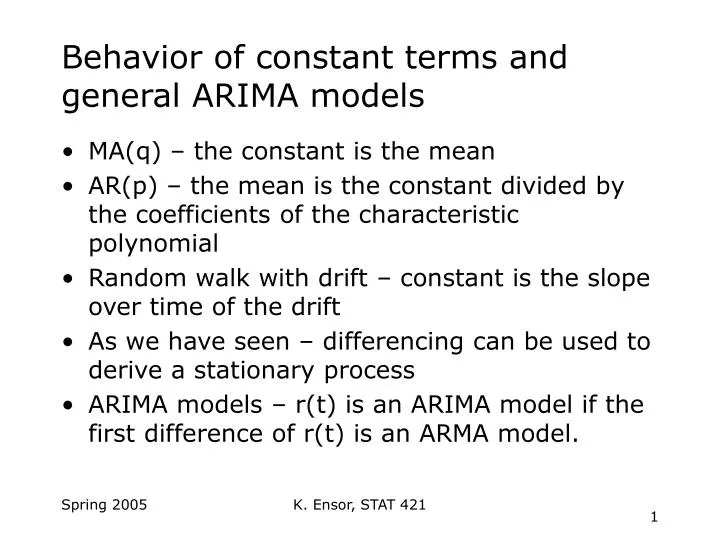
Behavior of constant terms and general ARIMA models • MA(q) – the constant is the mean • AR(p) – the mean is the constant divided by the coefficients of the characteristic polynomial • Random walk with drift – constant is the slope over time of the drift • As we have seen – differencing can be used to derive a stationary process • ARIMA models – r(t) is an ARIMA model if the first difference of r(t) is an ARMA model. K. Ensor, STAT 421
Unit-root nonstationary • Random walk p(t)=p(t-1)+a(t) p(0)=initial value a(t)~WN(0,2) • Often used as model for stock movement (logged stock prices). • Nonstationary • The impact of past shocks never diminishes – “shocks are said to have a permanent effect on the series”. • Prediction? • Not mean reverting • Variance of forecast error goes to infinity as the prediction horizon goes to infinity K. Ensor, STAT 421
Random Walk with Drift • Include a constant mean in the random walk model. • Time-trend of the log price p(t) and is referred to as the drift of the model. • The drift is multiplicative over time p(t)=t + p(0) + a(t) + … + a(1) • What happens to the variance? K. Ensor, STAT 421
Drift parameter= 0.5 Standard Deviation of shocks=2.0 K. Ensor, STAT 421
Drift parameter= 0.5 Standard Deviation of shocks=2.0 K. Ensor, STAT 421
Unit Root Tests • The classic test was derived by Dickey and Fuller in 1979. The objective is to test the presence of a unit root vs. the alternative of a stationary model. • The behavior of the test statistics differs if the null is a random walk with drift or if it is a random walk without drift (see text for details). K. Ensor, STAT 421
Unit root tests continued • There are many forms. The easiest to conceptualize is the following version of the Augmented Dickey Fuller test (ADF): • The test for unit roots then is simply a test of the following hypothesis: against • Use the usual t-statistic for testing the null hypothesis. Distribution properties are different. K. Ensor, STAT 421
Unit root tests • In finmetrics use the following command • Without finmetrics you will need to simulate the distribution under the null hypothesis – see the Zivot manual for the algorithm. • unitroot(rseries,trend="c",statistic="t", method="adf",lags=6) K. Ensor, STAT 421
Stationary Tests • Null hypothesis is that of stationarity. • Alternative is a non-stationary process. • Null hypothesis is that the variance of ε is 0. • In finmetrics use command stationaryTest(x, trend="c", bandwidth=NULL, na.rm=F) K. Ensor, STAT 421