AN alysis O f VA riance can be used to test for the equality of three or more population means.

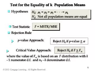
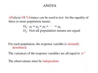
1. ANOVA • ANalysisOf VAriancecan be used to test for the equality of three or more population means. H0: 1=2=3=. . . = k Ha: Not all population means are equal normally For each population, the response variable is The variances of the response variables are all equal to The observations must be distributed.  2 independent.

2. ANOVA Sampling Distribution of x given H0 is true  Sample means are “close” together because there is only one sampling distribution when H0 is true.

3. ANOVA There are k treatments: For j = k 1 3 2 yada, yada, yada is computed from a random sample of size The overall sample mean: Dividing the following by k – 1 givens the MSTR

4. ANOVA There are k treatments: For j = k is computed from a random sample of size The overall sample mean: Dividing the following by k – 1 givens the MSTR

5. ANOVA Sampling Distribution of x when H0is false 3  2 1 Sample means come from different sampling distributions, and so are not as “close” together when H0 is false.

6. ANOVA There are k treatments: Forj = k 1 3 2 yada, yada, yada is computed from a random sample of size The overall total number of observations in all samples: nT = n1 + n2 + n3 + … + nk Dividing the following by nT – k givens the MSE

7. ANOVA There are k treatments: For j = k is computed from a random sample of size The overall total number of observations in all samples: nT = n1 + n2 + n3 + … + nk Dividing the following by nT – k givens the MSE

8. ANOVA The following is the SST which has nT – 1 degrees of freedom

9. ANOVA Source of Variation Sum of Squares Mean Squares Degrees of Freedom F SSTR SSE k – 1 nT – k Treatment Error Total MSE MSTR F-stat nT – 1 SST If F-stat is “small”… If F-stat is “BIG” … … you cannot reject H0 …we reject H0 The above ANOVA procedure is an example of a completely randomized design, and is applicable when • treatments are randomly assigned to the experimental units • useful when the experimental units are homogenous

10. Completely Randomized Design Example 1 Janet Reed would like to know if there is any significant difference in the mean number of hours worked per week for the department managers at her three manufacturing plants (in Buffalo, Pittsburgh, and Detroit). A simple random sample of five managers from each of the three plants was taken and the number of hours worked by each manager for the previous week is shown on the next slide. Conduct an F test at the 5% level of significance. NOTE: k = 3 and n1 = n2 = n3 = 5

11. Completely Randomized Design Average weekly hours worked by department managers Plant 3 Detroit Plant 2 Pittsburgh Plant 1 Buffalo Observation 1 2 3 4 5 48 54 57 54 62 51 63 61 54 56 73 63 66 64 74 ni 5 5 5 xi 55 68 57 26.0 26.5 24.5 si2

12. = (55 + 68 + 57)/3 = 60 Completely Randomized Design 1. Develop the hypotheses. H0:  1= 2= 3 Ha: Not all the means are equal 2. Determine the critical value Column k– 1 = 2 2 F.05 = 3.89 a= .05 Row: nT– k =12 3. Compute MSTR SSTR = 5(55 – 60)2 + 5(68 – 60)2 + 5(57 – 60)2 490 = 490 MSTR = = 245 /

13. 245 Completely Randomized Design 4. Compute the MSE SSE = 4(26.0) + 4(26.5) + 4(24.5) 308 = 308 MSE = 25.667 /(15 – 3) = nT k 5. Compute the F-stat / = 9.55 = F = MSTR/MSE

14. Completely Randomized Design Source of Variation Sum of Squares Mean Squares Degrees of Freedom F 490 308 2 12 245 Treatment Error Total 9.55 25.667 14 798 At 5% significance, the mean hours worked by department managers is not the same. Do Not Reject H0Reject H0 .05 3.89  1 9.55

15. ANOVA • Example: Crescent Oil Co. Crescent Oil has developed 3 new blends of gasoline and must decide which blend or blends to produce and distribute. A study of the MPG ratings of the 3 blends is being conducted to determine if the mean ratings are the same for the three blends at a 10% level of significance. Each of the 3 gasoline blends have been tested on 5 automobiles. The MPG ratings for the 15 automobiles are shown in the table on the next slide. If the experimental units are heterogeneous, use Randomized Block Design

16. Randomized Block Design Type of Gasoline (Treatment) Automobile (Block) Block Means Blend X Blend Y Blend Z 1 2 3 4 5 31 30 29 33 26 30 29 29 31 25 30 29 28 29 26 30.333 29.333 28.667 31.000 25.667 Treatment Means 29 29.8 28.8 28.4

17. Randomized Block Design + (30 – 29)2 SST = (31 – 29)2 + (30 – 29)2 + (29 – 29)2 + (30 – 29)2 + . . . . . . + (26 – 29)2 = 62 62 SSTR = (5)[] (29.8 – 29)2 + (28.8–29)2 + (28.4 – 29)2 = 5.2 5.2 SSBL = (3)[ ] (30.333 – 29)2 + (29.333 – 29)2 = 51.33 51.33 + (28.667 – 29)2 + (25.667 – 29)2 + (31.000 – 29)2 SSE = -- = 5.47 Most of the variation is across blocks

18. Randomized Block Design ANOVA Table Source of Variation Sum of Squares Degrees of Freedom Mean Squares F Treatments 5.20 2.60 3.82 2 Blocks 51.33 4 12.83 Error 5.47 8 .68 Total 62.00 14 NOTE: when the F-stat is “big” the estimated variances are “far apart”, and so the population means are probably different.

19. Randomized Block Design Row: denominator df = 8,a = .10 Column: numerator df = 2 At 10% significance, the MPG ratings differ for the three gasoline blends. Do Not Reject H0 Reject H0 .10 0 F 3.82 3.11  1 F-stat