Download

1 / 55
550 likes | 674 Views
16.360 Lecture 2. Transmission lines. Transmission line parameters, equations Wave propagations Lossless line, standing wave and reflection coefficient Input impedence Special cases of lossless line Power flow Smith chart Impedence matching Transients on transmission lines.

E N D
16.360 Lecture 2 • Transmission lines • Transmission line parameters, equations • Wave propagations • Lossless line, standing wave and reflection coefficient • Input impedence • Special cases of lossless line • Power flow • Smith chart • Impedence matching • Transients on transmission lines
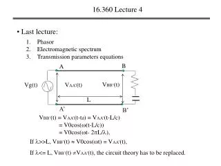
16.360 Lecture 2 • Transmission line parameters, equations B A VBB’(t) = VAA’(t) VBB’(t) Vg(t) VAA’(t) L A’ B’ VAA’(t) = Vg(t) = V0cos(t), Low frequency circuits: VBB’(t) = VAA’(t) Approximate result VBB’(t) = VAA’(t-td) = VAA’(t-L/c) = V0cos((t-L/c)),
B A VBB’(t) Vg(t) VAA’(t) L A’ B’ 16.360 Lecture 2 • Transmission line parameters, equations Recall: =c, and = 2 VBB’(t) = VAA’(t-td) = VAA’(t-L/c) = V0cos((t-L/c)) = V0cos(t- 2L/), If >>L, VBB’(t) V0cos(t) = VAA’(t), If <= L, VBB’(t) VAA’(t), the circuit theory has to be replaced.
B A VBB’(t) Vg(t) VAA’(t) L A’ B’ 16.360 Lecture 2 • Transmission line parameters, equations e. g: = 1GHz, L = 1cm Time delay t = L/c = 1cm /3x1010 cm/s = 30 ps Phase shift = 2ft = 0.06 VBB’(t) = VAA’(t) = 10GHz, L = 1cm Time delay t = L/c = 1cm /3x1010 cm/s = 30 ps Phase shift = 2ft = 0.6 VBB’(t) VAA’(t)
B A VBB’(t) Vg(t) VAA’(t) L A’ B’ 16.360 Lecture 2 • Transmission line parameters • time delay VBB’(t) = VAA’(t-td) = VAA’(t-L/vp), • Reflection: the voltage has to be treat as wave, some bounce back • power loss: due to reflection and some other loss mechanism, • Dispersion: in material, Vp could be different for different wavelength
B E 16.360 Lecture 2 • Types of transmission lines • Transverse electromagnetic (TEM) transmission lines B E a) Coaxial line b) Two-wire line c) Parallel-plate line d) Strip line e) Microstrip line
16.360 Lecture 2 • Types of transmission lines • Higher-order transmission lines a) Optical fiber b) Rectangular waveguide c) Coplanar waveguide
16.360 Lecture 2 • Lumped-element Model • Represent transmission lines as parallel-wire configuration A B Vg(t) VBB’(t) VAA’(t) B’ A’ z z z R’z L’z L’z R’z L’z R’z Vg(t) G’z C’z C’z C’z G’z G’z
16.360 Lecture 2 • Transmission line equations • Represent transmission lines as parallel-wire configuration i(z,t) i(z+z,t) L’z R’z V(z,t) V(z+ z,t) G’z C’z V(z,t) = R’z i(z,t) + L’z i(z,t)/ t + V(z+ z,t), (1) i(z,t) = G’z V(z+ z,t) + C’z V(z+ z,t)/t + i(z+z,t), (2)
i(z,t) i(z+z,t) L’z R’z V(z,t) V(z+ z,t) G’z C’z jt jt V(z,t) = Re( V(z) e i (z,t) = Re( i (z) e ), ), 16.360 Lecture 2 • Transmission line equations V(z,t) = R’z i(z,t) + L’z i(z,t)/ t + V(z+ z,t), (1) -V(z+ z,t) + V(z,t) = R’z i(z,t) + L’z i(z,t)/ t - V(z,t)/z = R’ i(z,t) + L’ i(z,t)/ t, (3) Rewrite V(z,t) and i(z,t) as phasors, for sinusoidal V(z,t) and i(z,t):
i(z,t) i(z+z,t) L’z R’z V(z,t) V(z+ z,t) G’z C’z jt e j = Re(i ), - dV(z)/dz = R’ i(z) + jL’ i(z), (4) 16.360 Lecture 2 • Transmission line equations Recall: jt di(t)/dt= Re(d i e )/dt - V(z,t)/z = R’ i(z,t) + L’ i(z,t)/ t, (3)
16.360 Lecture 2 • Transmission line equations • Represent transmission lines as parallel-wire configuration i(z,t) i(z+z,t) L’z R’z V(z,t) V(z+ z,t) G’z C’z V(z,t) = R’z i(z,t) + L’z i(z,t)/ t + V(z+ z,t), (1) i(z,t) = G’z V(z+ z,t) + C’z V(z+ z,t)/t + i(z+z,t), (2)
i(z,t) i(z+z,t) L’z R’z V(z,t) V(z+ z,t) G’z C’z jt jt V(z,t) = Re( V(z) e i (z,t) = Re( i (z) e ), ), 16.360 Lecture 4 • Transmission line equations i(z,t) = G’z V(z+ z,t) + C’z V(z+ z,t)/t + i(z+z,t), (2) - i (z+ z,t) + i (z,t) = G’z V(z + z ,t) + C’z V(z + z,t)/ t - i(z,t)/z = G’ V(z,t) + C’ V(z,t)/ t, (5) Rewrite V(z,t) and i(z,t) as phasors, for sinusoidal V(z,t) and i(z,t):
i(z,t) i(z+z,t) L’z R’z V(z,t) V(z+ z,t) G’z C’z jt e j = Re(V ), - d i(z)/dz = G’ V(z) + jC’ V(z), (7) 16.360 Lecture 2 • Transmission line equations Recall: jt dV(t)/dt= Re(d V e )/dt - i(z,t)/z = G’ V(z,t) + C’ V(z,t)/ t, (6)
i(z,t) i(z+z,t) L’z R’z V(z,t) V(z+ z,t) G’z C’z - d i(z)/dz = G’ V(z) + jC’ V(z), (7) - dV(z)/dz = R’ i(z) + jL’ i(z), (4) - d²V(z)/dz² = R’ di(z)/dz + jL’ di(z)/dz, (8) 16.360 Lecture 2 • Telegrapher’s equation in phasor domain Take d /dz on both sides of eq. (4)
- dV(z)/dz = R’ i(z) + jL’ i(z), (4) - d²V(z)/dz² = R’ di(z)/dz + jL’ di(z)/dz, (8) 16.360 Lecture 2 • Telegrapher’s equation in phasor domain - d i(z)/dz = G’ V(z) + jC’ V(z), (7) substitute (7) to (8) d²V(z)/dz² = (R’ + jL’) (G’+ jC’)V(z), or d²V(z)/dz² - (R’ + jL’) (G’+ jC’)V(z) = 0, (9) d²V(z)/dz² - ²V(z) = 0, (10) ² = (R’ + jL’) (G’+ jC’), (11)
i(z,t) i(z+z,t) L’z R’z V(z,t) V(z+ z,t) G’z C’z - d i(z)/dz = G’ V(z) + jC’ V(z), (7) - dV(z)/dz = R’ i(z) + jL’ i(z), (4) 16.360 Lecture 2 • Telegrapher’s equation in phasor domain Take d /dz on both sides of eq. (7) - d² i(z)/dz² = G’ dV(z)/dz + jC’ dV(z)/dz, (12)
- dV(z)/dz = R’ i(z) + jL’ i(z), (4) 16.360 Lecture 2 • Telegrapher’s equation in phasor domain - d i(z)/dz = G’ V(z) + jC’ V(z), (7) - d² i(z)/dz² = G’ dV(z)/dz + jC’ dV(z)/dz, (12) substitute (4) to (12) d² i(z)/dz² = (R’ + jL’) (G’+ jC’)i(z), or d² i(z)/dz² - (R’ + jL’) (G’+ jC’) i(z) = 0, (9) d² i(z)/dz² - ²i(z) = 0, (13) ² = (R’ + jL’) (G’+ jC’), (11)
= Re (R’ + jL’) (G’+ jC’) , = Im (R’ + jL’) (G’+ jC’) , 16.360 Lecture 2 • Wave equations d²V(z)/dz² - ²V(z) = 0, (10) d² i(z)/dz² - ²i(z) = 0, (13) = + j,
= Re (R’ + jL’) (G’+ jC’) , = Im (R’ + jL’) (G’+ jC’) , z -z z -z e e e e 16.360 Lecture 2 • Wave equations d²V(z)/dz² - ²V(z) = 0, (10) d² i(z)/dz² - ²i(z) = 0, (13) = + j, Solving the second order differential equation + - V(z) = V0 (14) + V0 + - + i(z) = I0 (15) I0
+ - - + - + and are related to V0 V0 I0 V0 V0 I0 and by characteristic impedance Z0. -z -z z z e e e e 16.360 Lecture 2 • Wave equations + - V(z) = V0 (14) + V0 + - + i(z) = I0 (15) I0 where: and are determined by boundary conditions.
+ - V(z) = V0 (14) + V0 + - + i(z) = I0 (15) I0 + - - V0 V0 + - - dV(z)/dz = R’ i(z) + jL’ i(z), (4) i(z) = ) - (V0 V0 = (R’ + jL’) i(z), (16) (R’ + jL’) -z -z z z -z z z -z e e e e e e e e - - + + - I0 I0 = = V0 V0 (R’ + jL’) (R’ + jL’) 16.360 Lecture 2 • Characteristic impedance Z0 recall: (17) (18)
(R’ + jL’) V0 = (R’ + jL’) (G’+ jC’) + I0 (R’ + jL’) (G’+j C’) - - + + - I0 I0 = = V0 V0 (R’ + jL’) (R’ + jL’) 16.360 Lecture 5 • Characteristic impedance Z0 (17) (18) Define characteristic impedance Z0 recall: + Z0 = =
+ - V(z) = V0 (14) + V0 + - + i(z) = I0 (15) I0 + V0 = (R’ + jL’) (G’+ jC’) Z0 + I0 (R’ + jL’) (G’+j C’) = -z z z -z e e e e 16.360 Lecture 5 • Summary: (19) (20)
jL’ = Z0 j C’ = (R’ + jL’) (G’+ jC’) j = L’C’ L’C’ (R’ + jL’) (G’+j C’) = 16.360 Lecture 5 • Example, an air line : R’ = 0 , G’ = 0 /, Z0 = 50, = 20 rad/m, f = 700 MHz L’ = ? and C’ = ? solution: = 50 = + j, = = 20 rad/m
= (R’ + j L’ ) (G’+ jC’) j = = L’C’ L’C’ 16.360 Lecture 5 • lossless transmission line : = + j, = (R’ + jL’) (G’+ jC’) If R’<< j L’ and G’ << jC’, = 0 lossless line
jL’ = Z0 j C’ = L’C’ L’C’ L’C’ (R’ + jL’) Z0 1 (G’+j C’) = 2/ = = 1 L’ = = Vp = / C’ 16.360 Lecture 2 • lossless transmission line : lossless line = 0 = 2/
+ - V(z) = V0 + V0 c 1 c 1 1 + = = = = = - + i(z) = I0 I0 Z0 = = = = L’C’ L’C’ rr rr L’C’ L’C’ L’ -jz jz -jz jz e e e e = C’ 16.360 Lecture 2 • For TEM transmission line : L’C’ = Vp • summary : Vp
B A Z0 VL Vg(t) Vi ZL l z = - l z = 0 + + + - - - V0 V0 V0 V0 V0 V0 + - V(z) = V0 + V0 + - + + - - VL iL - i(z) = V0 V0 V0 V0 V0 V0 Z0 Z0 Z0 Z0 Z0 Z0 i(z) V(z) z = 0 z = 0 - ZL Z0 -jz jz jz -jz e e e e = + ZL Z0 16.360 Lecture 5 • Voltage reflection coefficient : VL = = + - iL = = + ZL = = -
+ + + i0 V0 V0 i = - = - - - - i0 V0 V0 16.360 Lecture 5 • Voltage reflection coefficient : - ZL Z0 = + ZL Z0 • Current reflection coefficient : • Notes : • || 1, how to prove it? • If ZL = Z0, = 0. Impedance match, no reflection from the load ZL.
16.360 Lecture 2 • An example : A RL = 50 f = 100MHz Z0 = 100 A’ CL = 10pF z = 0 ZL = RL + j/CL = 50 –j159 - ZL Z0 = + ZL Z0
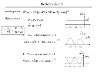
+ V0 with = - V0 + - V(z) = V0 + V0 - + + - i(z) = V0 V0 V0 jz jr Z0 Z0 Z0 e e jz jz -jz -jz -jz -jz jz -jz (e e e e e e e e + 1/2 = |V0| [1+ | |² + 2||cos(2z + r)] 16.360 Lecture 2 • Standing wave • Input impedance jz + e V(z) = V0() + - i(z) = ) + |V(z)| = |V0| || + ||
+ V0 with = - V0 + - V(z) = V0 + V0 - + + - i(z) = V0 V0 V0 jz jr Z0 Z0 Z0 e e jz jz -jz -jz -jz -jz jz -jz (e e e e e e e e + 1/2 = |V0| [1+ | |² + 2||cos(2z + r)] 16.360 Lecture 2 • Standing wave jz + e V(z) = V0() + - i(z) = ) + |V(z)| = |V0| || + ||
jz + e + - || + V0 jz jr Z0 e e jz -jz -jz -jz (e e e e + 1/2 = |V0| [1+ | |² + 2||cos(2z + r)] 16.360 Lecture 2 • Standing wave V(z) = V0() - i(z) = ) + |i(z)| = |V0| /|Z0||| + 1/2 = |V0|/|Z0| [1+ | |² - 2||cos(2z + r)] |V(z)|
|V(z)| + |V0| - -3/4 -/2 -/4 |V(z)| |V(z)| + 2|V0| + 1/2 - -3/4 -/2 -/4 = |V0| [1+ | |² + 2||cos(2z + r)] 16.360 Lecture 2 Special cases • ZL= Z0, = 0 + |V(z)| = |V0| 2. ZL= 0,short circuit, = -1 + 1/2 |V(z)| = |V0| [2 + 2cos(2z + )]
|V(z)| + 2|V0| |V(z)| - -3/4 -/2 -/4 + 1/2 = |V0| [1+ | |² + 2||cos(2z + r)] 16.360 Lecture 2 Special cases 3. ZL= ,open circuit, = 1 + 1/2 |V(z)| = |V0| [2 + 2cos(2z )]
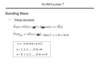
+ |V(z)| |V0| [1+ | |], = max |V(z)| + 1/2 = |V0| [1+ | |² + 2||cos(2z + r)] 16.360 Lecture 2 • Voltage maximum when 2z + r = 2n. –z = r/4+n/2 n = 1, 2, 3, …, if r <0 n = 0, 1, 2, 3, …, if r >= 0
+ |V(z)| |V0| [1 - | |], = min |V(z)| + 1/2 = |V0| [1+ | |² + 2||cos(2z + r)] 16.360 Lecture 2 • Voltage minimum when 2z + r = (2n+1). –z = r/4+n/2 + /4 Note: voltage minimums occur /4 away from voltage maximum, because of the 2z, the special frequency doubled.
S |V(z)| |V(z)| min max 1 + | | = 1 - | | 16.360 Lecture 2 • Voltage standing-wave ratio VSWR or SWR S = 1, when = 0, S = , when || = 1,
B A Z0 VL Vg(t) Vi ZL l z = - l z = 0 16.360 Lecture 2 • An example Voltage probe S = 3, Z0 = 50, lmin = 30cm, lmin = 12cm, ZL=? Solution: lmin = 30cm, = 0.6m, S = 3, || = 0.5, -2lmin + r = -, r = -36º, , and ZL.
jz jz + + e e + - ( ( ) ) V0 V0 V(z) I(z) j2z -j2l -j2l j2z e e e e - + - + (1 (1 (1 (1 ) ) ) ) Z0 Z0 -jz -jz e e 16.360 Lecture 2 • Input impudence B Ii A Zg Vg(t) Z0 VL Vi ZL l z = - l z = 0 Zin(z) = Z0 = = Zin(-l) =
-j2l -j2l e e - + (1 (1 ) ) Z0 16.360 Lecture 2 An example A 1.05-GHz generator circuit with series impedance Zg = 10- and voltage source given by Vg(t) = 10 sin(t +30º) is connected to a load ZL = 100 +j5- through a 50-, 67-cm long lossless transmission line. The phase velocity is 0.7c. Find V(z,t) and i(z,t) on the line. Solution: Since, Vp = ƒ, = Vp/f = 0.7c/1.05GHz = 0.2m. = 2/, = 10 . = (ZL-Z0)/(ZL+Z0), = 0.45exp(j26.6º) Zin(-l) = = 21.9 + j17.4 Zin(-l) + V0[exp(-jl)+ exp(jl)] Vg = Zin(-l) + Zg
+ V0 Z0 jz jz -jz -jz e (e e (e 16.360 Lecture 2 short circuit line B Ii A Zg Vg(t) sc Z0 VL Zin ZL = 0 l z = - l z = 0 ZL= 0, = -1, S = + V(z) = V0 ) - = -2jV0sin(z) + + i(z) = ) = 2V0cos(z)/Z0 V(-l) Zin = jZ0tan(l) = i(-l)
-1 l = 1/[- tan (1/CeqZ0)], 16.360 Lecture 2 short circuit line V(-l) Zin = jZ0tan(l) = i(-l) • If tan(l) >= 0, the line appears inductive, jLeq= jZ0tan(l), • If tan(l) <= 0, the line appears capacitive, 1/jCeq= jZ0tan(l), • The minimum length results in transmission line as a capacitor:
16.360 Lecture 2 An example: Choose the length of a shorted 50- lossless line such that its input impedance at 2.25 GHz is equivalent to the reactance of a capacitor with capacitance Ceq = 4pF. The wave phase velocity on the line is 0.75c. Solution: Vp= ƒ, = 2/ = 2ƒ/Vp = 62.8 (rad/m) tan (l)= - 1/CeqZ0 = -0.354, -1 l= tan (-0.354) + n, = -0.34 + n,
+ = 2V0cos(z) + V0 Z0 jz jz -jz -jz e (e e (e 16.360 Lecture 2 open circuit line B Ii A Zg Vg(t) oc Z0 VL Zin ZL = l z = - l z = 0 ZL= 0, = 1, S = + V(z) = V0 ) + - i(z) = ) = 2jV0sin(z)/Z0 V(-l) oc Zin = -jZ0cot(l) = i(-l)
oc sc Zin Zin • Measure and sc oc = -jZ0cot(l) = jZ0tan(l) Zin Zin oc sc sc oc Zin Zin Zin Zin Z0 = Z0 = -j 16.360 Lecture 2 Application for short-circuit and open-circuit • Network analyzer • Measure S paremeters • Calculate Z0 • Calculate l
-j2l -j2l e e + - (1 (1 ) ) Z0 16.360 Lecture 2 Line of length l = n/2 tan(l) = tan((2/)(n/2)) = 0, Zin(-l) = = ZL Any multiple of half-wavelength line doesn’t modify the load impedance.
(1 - ) Z0 (1 + ) -j2l -j2l e e - + (1 (1 ) ) Z0 16.360 Lecture 2 Quarter-wave transformer l = /4 + n/2 l = (2/)(/4 + n/2) = /2 , -j e + ) (1 Zin(-l) = = Z0 = -j e - (1 ) = Z0²/ZL
16.360 Lecture 2 An example: A 50- lossless tarnsmission is to be matched to a resistive load impedance with ZL = 100 via a quarter-wave section, thereby eliminating reflections along the feed line. Find the characteristic impedance of the quarter-wave tarnsformer. Z01 = 50 ZL = 100 /4 Zin = Z0²/ZL= 50 ½ ½ Z0 = (ZinZL) = (50*100)