Download

1 / 107
1.07k likes | 1.08k Views
The ACE Grain Flow Model: Background, Model and Data. February 14 2007, To the Navigation Economic Technologies (NETS) Grain Forecast Modeling and Scenarios Workshop , By Dr. William W Wilson and Colleagues DeVuyst, Taylor, Dahl and Koo bwilson@ndsuext.nodak.edu.

E N D
The ACE Grain Flow Model: Background, Model and Data February 14 2007, To theNavigation Economic Technologies (NETS) Grain Forecast Modeling and Scenarios Workshop, By Dr. William W Wilson and Colleagues DeVuyst, Taylor, Dahl and Koo bwilson@ndsuext.nodak.edu
Paper/reports are as follow • Available at WWW/nets • Longer-Term Forecasting of Commodity Flows on the Mississippi River: Application to Grains and World Trade • Appendix titled Longer-Term Forecasting of Commodity Flows on the Mississippi River: Application to Grains and World Trade: Appendix • IWR Report 006-NETS-R-12 • http://www.nets.iwr.usace.army.mil/docs/LongTermForecastCommodity/06-NETS-R-12.pdf • NDSU Research Reports forthcoming
Outline of Topics: ACE I • Background • Model description • Summary of critical data • ACE II: Additional restrictions, calibration, results and summary
Analytical Challenge and Background • Panama Canal Expansion Project and Analysis • Simply expand/update/revise • Data: Needed to be replicatable/ observable and scientifically defendable • Focus two extreme scopes of analysis in one • Extreme detail on US intermodal competition including inter-reach competition! • Macro trade and policies • 50 year projections
Overall Approach • Data • Assumptions • Model • Results
NAS Review: Key Points and Major Changes • Drop wheat from model • Supply/Demand data. Data updated to most recent available • Domestic demand by crop and state: Use ProExporter data. Comment on USDA • Ethanol. Data and related issues updated and more detail • Barge rates: replaced means with barge rate functions • Brazil shipping costs. revised using shipping costs concurrent with base period and which are now reported in USDA Grain Transportation. • Interior shipping restrictions Restrictions on port/river handling were removed (notably STl and NOrleans) • Rail car capacity was added as a restriction, • Truck rates. Shipping rates to the river were revised and taken from Dager (forthcoming). • Calibration: • extensive comparisons of model results to actual rail and barge shipments during the base period. • When/if there was a difference, we compared the elements of costs to identify the reasons for this difference. • Selectively imposed restrictions to reduce the number of flows that did not conform to actual. These are summarized on p. 11 of the Appendix (and below)
Model Dimensions and Scope Major components of the model • Consumption and import demand: • Estimates of consumption were generated based on incomes, population and the change in income elasticity as countries mature. For the United States, ethanol demand for corn was treated separately from other sources of demand. • Export supply: For each exporting country and region, export supply is defined as the residual of production and consumption. • Costs Included: • Production (Variable) costs • Shipping by truck, rail, barge and ocean • Barge delay costs (nonlinear) • Handling costs • Import tariffs, export subsidies and trade restrictions • Model dimensions: The model was defined in GAMS and has • 21,301 variables • 761 restrictions.
Model Details • Production calculations • Max area potential: • HA=f(trend) • Total area subject to max % increase from base period • Max switching between crops: • 12% (base) -20% • Yields=f(trend) • Model chooses least cost solution and derives • Area planted to each crop by region • Production • Consumption • Trade • Route, inter-reach allocation and intermodal allocation
Other restrictions: Wheat • Due to a cumulation of peculiarities on wheat trade and marketing, mostly due to cost differentials and quality demands • imposed a set of restrictions to • ensure countries’ trade patterns were represented • allow some inter-port area shifts in flows within North America • Allow growth to occur with similar shares
Other • Base case and other restrictions discussed in ACE 2 (concurrent with results)
Background: Data and Observations Impacting results • Consumption • Production costs • Yields, CRP etc. • Ethanol
Consumption Functions • Changes in consumption as countries’ incomes increase • Econometrics: • C=f(Y) • C=consumption and Y=income • For each country and commodity using time series data • Use to generate elasticity for each country/commodity • E=f(Y) • E= Elasticity • Non-linear • Across cross section of time series elasticity estimates • Allow elasticities for each country to change as incomes increase • Derive projections • Use WEFA income and population estimates • Derive consumption as • C=C+%Change in Y X Elasticity
Estimated Income Elasticities for Selected Countries/Regions
Wheat: Forecast Consumption, Selected Countries/Regions, 2005-2050
Corn: Forecast Consumption, Selected Countries/Regions, 2005-2050
Soybean: Forecast Consumption, Selected Countries/Regions, 2005-2050
Grain/Oilseed Production Cost • Data from Global Insights • By country and crop • Standardized method to derive variable costs/HA • Combined with estimated yields to derive costs in $/mt • By crop • By country/region • Projections
Cost advantage for U.S. producing regions diminishes over time • Increases in production costs for U.S. regions rise at similar rates to that for major competing exporters. • The rate of increase in yields in US is less (slightly) than competing exporters. • In competing countries, the rate of increase in yields is comparable to that of production costs. • In the United States, yield increases are less than competing exporters’; and, are less than production cost increases. • The impact of these is very subtle, but, when extrapolated forward, results in a changing competitive position of the United States relative to competing countries.
Ethanol • Projections and sensitivities • EIA 2005 was the base case • EIA 2006 assumption (Ethanol sensitivity) • Qualified alternative stylized assumptions • Method • Current known demand: Assumed • New demand: • Allocated proportionately across states • DDGs produced • returned to regional feed demand proportionate to its value
Newly announced plants (July 2006) • Illinois: • 7 plants and 30 in various planning stages • Iowa: • 24 operating units in Iowa • Nebraska: • 12 plants and about 22 in planning stages • North Dakota : 4 projects underway • Hankinson, Red Tail Energy, Spiritwood Underwood and Williston (announced in Williston on July 7, 2006).
Plans for new plants and expansions continue to change • Iowa exported 803 million bushels in 2003, but by 2008 would be deficit 400-500 million bushels with existing plants running at rated capacity (Wisner); • ProExporter estimates were 5.3 billion gallons of capacity currently operating, and another 6 billion under construction. • There were an additional 369 projects on the drawing boards representing an additional 24.7 bill gallons of ethanol capacity (as Ethanol margins in 2005 was 152 c/bu of corn processed and this has declined to 44 c/bu this year, and this was more than attractive to justify additional investment. • Goldman Sach expressed worry about high corn prices indicating that rising corn prices threaten profitability of ethanol. Biomargins have been hurt by 55% increase in corn price and price of ethanol has risen by 8%. Without producer incentives and tax credits Goldman believes many biofuel plants would be unprofitable.
ProExporter Blue-Sky Model • Longer term • Ethanol use would converge to 18.7 billion gallons • In the US • Corn production would be • Exports would be • Origination wars in Minnesota, Iowa and Nebraska as shuttle shippers for feed to California and the Southwest, and the PNW have to compete with ethanol. • Due to superior margins in ethanol, the latter would set the price and force others to pay more.
CARD/ISU Study • Results indicated the break-even corn price is 405c/b. • Corn based ethanol would increase to 31.5 bill gal by 2015. • U.S. would have to plant 95.6 million acres of corn (vs. 79 million in 2006) and produce 15.6 bill bush (vs. 11 billion today). • Most of the acres would come from reduced soybean acreage. • There would be a 9 million-acre reduction in soybean area • a change in rotation from corn-soybean to corn-corn-soybean. • Corn exports would be reduced substantially and suggested the U.S. could become a corn importer. • Finally, wheat prices would increase 20% • there would be a 3% reduction in wheat area with wheat feed use increasing • Wheat exports decline 16 percent.