Download

1 / 36
360 likes | 471 Views
Disc Covering Problem with Application to Digital Halftoning. Dagstuhl Workshop, 2004. Tetsuo Asano School of Information Science, JAIST Japan Advanced Institute of Science and Technology Joint Work with Shinji Sasahara , Fuji Xerox Co.Ltd. Peter Brass , CUNY, U.S.A.

E N D
Disc Covering Problem with Application to Digital Halftoning DagstuhlWorkshop, 2004 Tetsuo Asano School of Information Science, JAIST Japan Advanced Institute of Science and Technology Joint Work with Shinji Sasahara, Fuji Xerox Co.Ltd. Peter Brass, CUNY, U.S.A.
Problem Specification Problem: R = {r11, r12, ... , rnn} : a matrix of n2 positive real numbers. Each rij is a radius of a disc at (i,j). Choose disks so as to maximize the total singly-covered area. R= circle of radius 1.2 singly-covered area
Example: a set of input discs given by a matrix a set of discs that maximizes the total singly-covered area
a set of discs singly-covered area
Algorithmic questions and Motivation: • How hard is it? NP-hard? • Approximation algorithm with guaranteed ratio • One-dimensional problem still hard? or an efficient algorithm? • Motivation application to digital halftoning: conversion from continuous-tone images to binary-tone images
How hard is it? NP-hard? • NP-hard or polynomial-time algorithm? open • One-dimensional problem still hard? or an efficient algorithm? polynomial-time algorithms 1. graph-based approach 2. plane-sweep and dynamic programming
Approximation algorithm with guaranteed performance Cu: a disc with center at u r(Cu): radius of the disc Cu Cu u Algorithm 1: ・Sort all the discs in the decreasing order of their radii. ・for each disc Cu in the order do ・ if Cu does not intersect any previously accepted disc ・ then accept it else reject it ・Output all the accepted discs.
accepted discs by Algorithm 1 input set of discs
Cu: a disc which has not been accepted by Algorithm 1 • there must be some disc Cv such that (1) Cv has been examined before Cu, and (2) Cv intersects Cu. Cu Cv (1) r(Cv)≧r(Cu) : larger discs are examined first If we enlarge Cv by a factor 3, the all the discs rejected by Cv are completely contained in the enlarged disc. Lemma 5: Algorithm 1 finds a 9-approximate solution. Proof: S: a set of all input discs S’: a solution (set of discs) obtained by Algorithm 1. all the discs in S’ are disjoint.
Rr(Cv) Cv Rr(Cu) Cu Cv violates Cu if Cv intersects the core Rr(Cu) of Cu. Otherwise, two discs safely intersect. Approximation algorithm with better performance some terminologies and notations: Cu: a disc with center at u r(Cu): radius of the disc Cu Rr(Cu): a disc contracted by r, 0<r<1, which is called the core of the disc Cu. In this case Cv violates Cu but Cu does not violates Cv
Algorithm 2: ・Sort all the discs in the decreasing order of their radii. ・for each disc Cu in the order do ・ if Cuis not violated by any previously accepted disc (i.e., Cu does not intersect the core of any previously accepted disc) ・ then accept it else reject it ・Output all the accepted discs. Rr(Cv) Cv Rr(Cu) in this case Cu can be accepted Cu
input set of discs accepted discs
Lemma 6: Algorithm 2 finds a 5.83-approximate solution. Proof: • Cu: a disc which has not been accepted by Algorithm 2 • there must be some disc Cv such that (1) Cv has been examined before Cu, and (2) Cv violates Cu i.e., Cv intersects the core of Cu. Rr(Cv) Cv Rr(Cu) Cu Enlarge each accepted disc by a factor 2 + r
Enlarge each accepted disc by a factor 2 + r Rr(Cv) Cv Rr(Cu) Cu Every disc rejected by Cv is completely contained in the enlarged disc. How much area is covered exactly once by accepted discs?
How much area is covered exactly once by accepted discs? a set of accepted discs additively weighted Voronoi diagram of the discs truncate each Voronoi cell of an accepted disc by its blown-up copy evaluate how much area in each cell is covered by the disc ratio > 1 / 5.83.
blow up a disc by 2+r truncate each cell by the copy partition into angular sectors additively weighted Voronoi diagram of the discs accepted discs
Voronoi edge outside disc In this angular sector, at least 1/(2+r)2 is occupied by the disc. 2+r 1 Voronoi edge inside disc The core is not overlapped by any other disc. So, the ratio is at least r2.
Voronoi edge outside disc In this angular sector, at least 1/(2+r)2 is occupied by the disc. Voronoi edge inside disc The core is not overlapped by any other disc. So, the ratio is at least r2. We choose r so that r2= 1 / (2+r)2. Then, the ratio of singly-covered area is at least 1/(2+r)2. approximation ratio is (2+r)2=5.83.
NP-hardness proof (uncompleted) reduction from planar 3SAT variable part we have to choose either all of red circles or all of blue circles.
NP-hardness proof(continued) path part
NP-hardness proof(continued) clause part
Open Problems • Improve the approximation ratio approximation ratio 2 or (1+e)? O(n log n) time and O(n) space for practical applications • Complete NP-hardness proof
Concluding Remarks considered a geometric optimization problem to choose discs among n given discs to maximize the singly-covered area. Application: adaptive digital halftoning. Proposed some heuristic algorithms and verified their effectiveness by experiments.
Heuristic Algorithm 1 (1) Fix a contraction factorr appropriately. (2) D = a set of all discs in the raster order (3) for each disc C in D (in raster order) accept C if core(C) does not intersect the core of any previously accepted disc and reject it otherwise. Rr(Cv) Cv Rr(Cu) Cu In this algorithm, the first disc in the raster order is always accepted, which may be a bad choice for future selection.
Heuristic Algorithm 2 (1) Fix a contraction factorr appropriately. (2) D = a set of all discs in the decreasing order of their radii (3) for each disc C in D (large discs first) accept C if core(C) does not intersect the core of any previously accepted disc and reject it otherwise. Rr(Cv) Cv Rr(Cu) Cu
Experimental Results Input images small: 106 x 85, and large: 256 x 320 enlarge them into 424 x 340 and 1024 x 1280
Running time Heuristic 1: 0.06 sec. for the small image 0.718 sec. for the large image on PC: DELL Precision 350 with Pentium 4. Heuristic 2: 0.109 sec. for the small image 1.031 sec. for the large image
Fill out each Voronoi cell according to the grey level at the center point of the cell by cubic interpolation