Download
1 / 23
380 likes | 1.12k Views
Surface Waves. Chris Linton. A (very loose) definition. A surface wave is a wave which propagates along the interface between two different media and which decays away from this interface. decay. direction of propagation. decay. Mathematical preliminaries.

E N D
Surface Waves Chris Linton
A (very loose) definition A surface wave is a wave which propagates along the interface between two different media and which decays away from this interface decay direction of propagation decay
Mathematical preliminaries • linear theory (small oscillations) • time-harmonic motion F(x,t) = Re[ f(x) e-iwt] wis the angular frequency (w/2pis in Hz) • f(x)is complex – it describes both the amplitude and phase of the wave • eikx represents a wave travelling in the x-direction with wavelength l = 2p/k
Water waves gravity fluid velocity -w2f + gfz + (s/r)fzzz= 0 u(x) = f(x) surface tension z x Laplace’s equation 2f =0 decay
z f = eikxekz try x dispersion relation w2 = gk + sk3/r g≅ 9.8 ms-1, water: r≅ 1000 kgm-3, s≅ 0.07 Nm-2 1 ms-1 speed c = w/k wavelength, l = 2p/k 17 mm 50 cm
Elastic waves In an infinite elastic solid, two types of waves can propagate u = uL+ uT =f + ×y longitudinal (P) waves, speed cL cT < cL transverse (S) waves, speed cT In rock, cL ≅ 6 kms-1,cT ≅ 3.5 kms-1,
Rayleigh waves zero traction f = Aeikxekaz z x y = (0,Beikxekbz,0) Navier’s equation decay u is in the (x,z)-plane • Surface waves exist, with speed cR < cT (< cL) • The quantity g =(cR/cT)2 satisfies the cubic equation • g3 - 8g2 + 8g(3-2L) - 16(1-L) = 0 • When L = 1/3, we find that cR≅ 0.9cT • Non-dispersive (cR does not depend on w)
Earthquakes Lord Rayleigh (1885) “It is not improbable that the surface waves here investigated play an important part in earthquakes” Rayleigh wave Love wave http://www.yorku.ca/esse/veo/earth/sub1-10.htm
SAW devices In the 1960s it was realised that Surface Acoustic Waves (Rayleigh waves) could be put to good use in electronics There are many types of SAW device They are used, e.g., in radar equipment, TVs and mobile phones Worldwide, about 3 billion SAW devices are produced annually http://tfy.tkk.fi/optics/research/m1.php
Electromagnetic surface waves e,m E = Êeilz, H = Ĥeilz x e,m Maxwell’s equations show that the field is determined from Êz and Ĥz. Both satisfy the Helmholtz equation z y Tangential components of E and H must be continuous on r = (x2+y2)1/2 = a 2u+(k2-l2)u=0 k2 = emw2/c2 k’2 = e’m’w2/c2 Require decay as r∞
Single mode optical fibres Try Êz = A Jm(ar) eimq, a2 = k2-l2 k2 < l2 < k2 B Km(a r) eimq, a2 = l2-k2 m = 0,1,2,… Except when m = 1, there is a critical radius below which waves of a given frequency cannot propagate The exception is often called the HE1,1 mode and single mode optical fibres can be fabricated with diameters of the order of a few microns Theory 1910, practical importance 1930s & 1940s, realisation 1960s
Edge waves z Kf = fz K = w2/g Stokes (1846) x f = eilye-l(x cos a – z sin a) a 2f =0 dispersion relation K = l sin a fn= 0 decay rigid boundary Extended by Ursell (1952) K = l sin (2n+1)a (2n+1)a < p/2 A continental shelf mode. From Cutchin & Smith, J. Phys. Oceanogr. (1973)
Array guided surface waves 1D array in 2D decay 1D array in 3D 2D array in 3D decay waves exist due to the periodic nature of the geometry Barlow & Karbowiak (1954)
McIver, CML & McIver (1998) 1D array in 2D a = 0.25, k = w/c = 2.5, b = 2.59 acoustic waves, rigid cylinders 2f +k2f = 0 quasiperiodicity f(x+1,y) = eibf(x,y) antisymmetric modes are also possible det(dmn+Zmsn-m(b)) = 0
dispersion curves, symmetric modes a = 0.125 a = 0.25 a = 0.375 k 0 < k < b ≤ p b
Excitation of AGSWs Thompson & CML (2007)
AGSWs on 2D lattices in 3D quasiperiodicity Rpq = ps1+qs2 f(r+Rpq) = eiRpq.bf(r) b is the Bloch vector s2 s1 det(dmn+Zmsn-m(b)) = 0 b can be restricted to the ‘Brillouin zone’ and we require |b| > k
s1 = (1,0), s2 = (0.2,1.2), k = 2.8, a = 0.3, arg b = p/4, |b|= 2.807 Thompson & CML (2010) in plane out of plane
Water waves over periodic array of horizontal cylinders eilydependence Kf = fz K = w2/g decay fn= 0 on rj=a (2–l2)f =0
bd – ld dispersion curves f/d=0.5, a/d=0.25, Kd=2,3,4,5,6,7 energy propagates normal to these isofrequency curves in the direction of increasing K
Transmitted energy over a finite array 41° 43° 50° CML (2011) 45° 49° 47° Kd=4, f/d=0.5, a/d=0.25 band gap for Kd=4 corresponds to ld in (2.808,3.017), or angle of incidence between 44.6 and 49.0 degrees
Summary • Surface waves occur in many physical settings • Mathematical techniques that can be used to analyse surface waves are often applicabe in many of these different contexts • There is often a long time between the theoretical understanding of a particular phenomenon and any practical use for it • The study of array guided surface waves is in its infancy