Download
1 / 36
470 likes | 875 Views
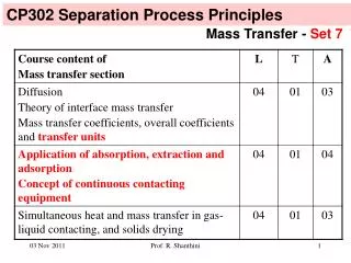
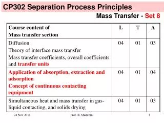
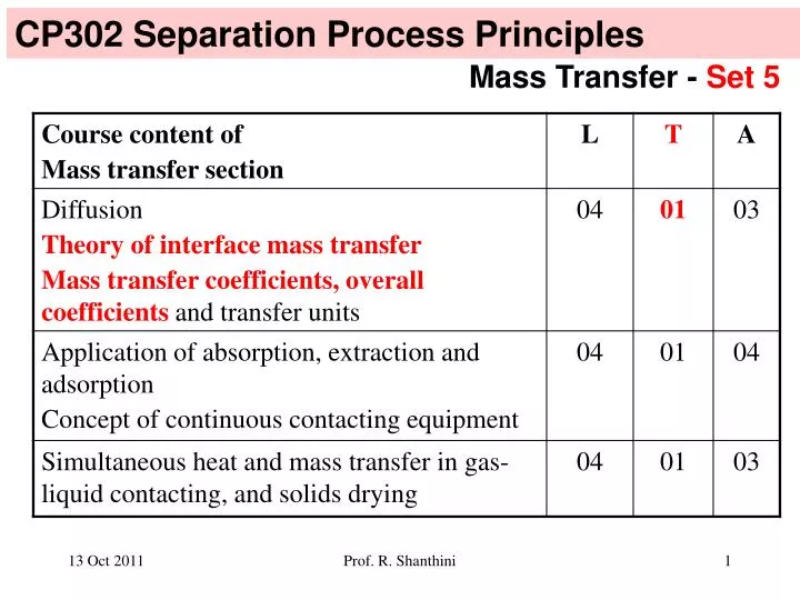
CP302 Separation Process Principles. Mass Transfer - Set 5. Summary: Two Film Theory applied at steady-state. = K G ( p Ab - p A * ) = K L (C A * - C Ab ). N A = k p (p Ab – p Ai ) = k c (C Ai – C Ab ). (52). (51). (59). (62). p Ai = H A C Ai. (53). Liquid film.

E N D
CP302 Separation Process Principles Mass Transfer - Set 5 Prof. R. Shanthini
Summary: Two Film Theory applied at steady-state = KG (pAb- pA*) = KL (CA*- CAb) NA = kp (pAb – pAi) = kc (CAi – CAb ) (52) (51) (59) (62) pAi = HA CAi (53) Liquid film Gas film pAb= HA CA* (60) pA*= HACAb (57) Liquid phase pAb pAi 1 HA 1 HA Gas phase = = + CAi KG KL kp kc CAb (58 and 61) Prof. R. Shanthini Mass transport, NA
Summary equations with mole fractions = Ky (yAb- yA*) = Kx (xA*- xAb) NA = ky (yAb – yAi) = kx (xAi – xAb ) (63) yAi = KA xAi (64) Liquid film Gas film yAb= KA xA* (65) yA*= KAxAb (66) Liquid phase yAb yAi 1 KA 1 KA Gas phase = = + (67) xAi Ky Kx ky kx xAb Prof. R. Shanthini Mass transport, NA
Notations used: xAb : liquid-phase mole fraction of A in the bulk liquid yAb : gas-phase mole fraction of A in the bulk gas xAi : liquid-phase mole fraction of A at the interface yAi : gas-phase mole fraction of A at the interface xA* : liquid-phase mole fraction of A which would have been in equilibrium with yAb yA* : gas-phase mole fraction of A which would have been in equilibrium with xAb kx : liquid-phase mass-transfer coefficient ky : gas-phase mass-transfer coefficient Kx : overall liquid-phase mass-transfer coefficient Ky : overall gas-phase mass-transfer coefficient KA : vapour-liquid equilibrium ratio (or equilibrium distribution coefficient) Prof. R. Shanthini
Gas-liquid equilibrium ratio (KA) curve yA yAb yAb = KAxA* yAi yAi = KA xAi yA* yA* = KA xAb xAb xAi xA* xA Prof. R. Shanthini
Gas-liquid equilibrium ratio (KA) curve yA How to determine KA? yAi yAi = KA xAi xAi xA Prof. R. Shanthini
Gas-liquid equilibrium ratio (KA) curve - nonlinear yA yAb yAb- yAi slope my = xA *- xAi yAi yAi- yA* yA* slope mx = xAi- xAb xAb xAi xA* xA Prof. R. Shanthini
Gas-liquid equilibrium ratio curve (is not linear) yA when driving forces for mass transfer are large yAb yAb- yAi slope my = xA *- xAi 1 1 1 yAi = + (67) Kx kx myky yAi- yA* yA* slope mx = xAi- xAb 1 1 mx = + (68) xAb xAi xA* xA Ky ky kx Prof. R. Shanthini Derivation is available on page 109 of Reference 2
1/kp 1/kp kc = = = 1/KG 1/kp + H/kc kc + H kp 1/kc 1/kc kp 1 1 = = 1 1 H 1 = 1/KL 1/Hkp + 1/kc kp + kc/H = = + + KG KL H kp kp kc kc Gas & Liquid-side Resistances in Interfacial Mass Transfer fG = fraction of gas-side resistance fL = fraction of liquid-side resistance Prof. R. Shanthini
Gas & Liquid-side Resistances in Interfacial Mass Transfer If fG > fL, use the overall gas-side mass transfer coefficient and the overall gas-side driving force. If fL > fG use the overall liquid-side mass transfer coefficient and the overall liquid-side driving force. Prof. R. Shanthini
1 HA 1 HA = = + (58 and 61) KG KL kp kc The above is also written with the following notations: 1 H 1 H = = + KOG KOL KG KL Prof. R. Shanthini
Tutorial discussed. Drive the relationship between the following under ideal conditions: (i) kp and ky (ii) kc and kx (iii) KG and Ky (iv) KL and Kx (v) HA and KA Prof. R. Shanthini
(i) Drive the relationship between kp and ky Start from NA = kp (pAb – pAi) = ky (yAb – yAi) (yAb – yAi) Therefore, kp = ky (pAb – pAi) Since, the partial pressure (pA) can be related to the mole fraction in vapour phase (yA) and the total pressure in the vapour phase (P) by pA = yA P for an ideal gas, the above expression can be rewritten as follows: (yAb – yAi) kp = ky = ky / P (yAb P – yAi P) Therefore ky = kp P (69) Prof. R. Shanthini
(ii) Drive the relationship between kc and kx Start from NA = kc (CAi – CAb) = kx (xAi – xAb) (xAi – xAb) Therefore, kc = kx (CAi – CAb) Since, the concentration (CA) can be related to the mole fraction in liquid phase phase (xA) and the total concentration in the liquid phase (CT) by CA = xA CT, the above expression can be rewritten as follows: (xAi – xAb) kc = kx = kx / CT (xAi CT– xAb CT) Therefore kx = kc CT (70) Prof. R. Shanthini
(iii) Drive the relationship between KG and Ky Start from NA = KG (pAb – pA*) = Ky (yAb – yA*) (yAb – yA*) Therefore, KG = Ky (pAb – pA*) using pA = yA P for an ideal gas, the above expression can be rewritten as follows: (yAb – yA*) KG = Ky = Ky / P (yAb P – yA* P) Therefore Ky = KG P (71) Prof. R. Shanthini
(iv) Drive the relationship between KL and Kx Start from NA = KL (CA*– CAb) = Kx (xA*– xAb) (xA*– xAb) Therefore, KL = Kx (CA*– CAb) Since CA = xA CT, the above expression can be rewritten as follows: (xA*– xAb) KL = Kx = Kx / CT (xA*CT– xAb CT) Therefore Kx = KL CT (72) Prof. R. Shanthini
(v) Drive the relationship between HA and KA Start from the equilibrium relationship pAi = HA CAi Since pAi = yAi P and CAi = xAi CT, the above expression can be written as follows: yAi P = HA xAi CT We know yAi = KA xAi Combining the above, we get the following: KA xAiP = HA xAi CT Therefore KA= HA CT/ P (73) True ONLY for dilute system Prof. R. Shanthini
Example on calculating Henry’s constant: Use the NH3-H2O data at 293 K given in the table below to calculate the Henry’s law constant (HA = pA / xA) at low concentrations of NH3, where pA is the equilibrium partial pressure of ammonia over aqueous solution having xA mole fraction of ammonia. Prof. R. Shanthini
Solution to Example on calculating Henry’s constant: The mass concentration data given in the table must be converted to mole fraction of ammonia in the liquid. It is done as follows: xA = (moles A) / (moles A + moles water) = (mA / MA) / [(mA / MA) + mH2O / MH2O)] = (20 / 17) / [(20 / 17) + 100 / 18)] for the first data point = 0.175 Prof. R. Shanthini
Solution to Example on calculating Henry’s constant: Prof. R. Shanthini
Solution to Example on calculating Henry’s constant: HA = 591 mm Hg per mol fraction of NH3 in water Prof. R. Shanthini
Solution to Example on calculating Henry’s constant: HA = 591 mm Hg per mol fraction of NH3 in water HA = 591 mm Hg mole fraction of NH3 in water Henry’s law constant determined above is HA = pA / xA. Use the relationship pA = yA PT, where pA is the partial pressure of NH3 in air, yA is the mol fraction NH3 in air and PT is the total pressure. Henry’s law constant therefore becomes HA = yA PT / xA, from which we get KA = yA / xA = HA/PT At 1 atm total pressure, KA = 591 / 760 = 0.778 mol fraction NH3 in air / mol fraction NH3 in water Prof. R. Shanthini
Example 1 Prof. R. Shanthini
Example 2 Prof. R. Shanthini
Example 3 Prof. R. Shanthini
Example 4 Prof. R. Shanthini