Download
1 / 50
500 likes | 656 Views
CPU Scheduling. Basic Concepts Scheduling Criteria Scheduling Algorithms First-Come-First-Served Shortest-Job-First, Shortest-remaining-Time-First Priority Scheduling Round Robin Multi-level Queue Multi-level Feedback Queue Real-Time CPU Scheduling. Basic Concepts.

E N D
CPU Scheduling • Basic Concepts • Scheduling Criteria • Scheduling Algorithms • First-Come-First-Served • Shortest-Job-First, Shortest-remaining-Time-First • Priority Scheduling • Round Robin • Multi-level Queue • Multi-level Feedback Queue • Real-Time CPU Scheduling GMU – CS 571
Basic Concepts • During its lifetime, a process goes through a sequence of CPU and I/O bursts. • In a multi-programmed computer system, multiple process compete for the CPU at a given time, to complete their current CPU bursts. GMU – CS 571
Basic Concepts • The CPU scheduler (a.k.a. short-term scheduler) will select one of the processes in the ready queue for execution. • The CPU scheduler algorithm may have tremendous effects on the system performance • Interactive systems • Real-time systems • Dispatcher module gives control of the CPU to the process selected by the short-term scheduler; this involves: • switching context • switching to user mode • jumping to the proper location in the user program to restart that program GMU – CS 571
Terminated New Admit Exit Scheduler Dispatch Ready Running Timeout Event occurs Event wait Waiting When to Schedule? Under a simple process state transition model, CPU scheduler could be invoked at five different points: 1. When a process switches from the new state to the ready state. 2. When a process switches from the running state to the waiting state. 3. When a process switches from the running state to the ready state. 4. When a process switches from the waiting state to the ready state. 5. When a process terminates. GMU – CS 571
Non-preemptive vs. Preemptive Scheduling • Under non-preemptive scheduling, each running process keeps the CPU until it completes or it switches to the waiting (blocked) state (points 2 and 5 from previous slides). • Under preemptive scheduling, a running process may be also forced to release the CPU even though it is neither completed nor blocked. • In time-sharing systems, when the running process reaches the end of its time quantum (slice) • In general, whenever there is a change in the ready queue. • Tradeoffs? GMU – CS 571
Scheduling Criteria • Several criteria can be used to compare the performance of scheduling algorithms • CPU utilization – keep the CPU as busy as possible • Throughput – # of processes that complete their execution per time unit • Turnaround time – amount of time to execute a particular process • Waiting time – amount of time a process has been waiting in the ready queue • Response time – amount of time it takes from when a request was submitted until the first response is produced, not the complete output. • Meeting the deadlines (real-time systems) GMU – CS 571
Optimization Criteria • Maximize the CPU utilization • Maximize the throughput • Minimize the (average) turnaround time • Minimize the (average) waiting time • Minimize the (average) response time • Minimize variance • In the examples, we will assume • average waiting time is the performance measure • only one CPU burst (in milliseconds) per process GMU – CS 571
First-Come, First-Served (FCFS) Scheduling • Single FIFO ready queue • No-preemptive • Not suitable for timesharing systems • Simple to implement and understand • Average waiting time dependant on the order processes enter the system GMU – CS 571
First-Come, First-Served (FCFS) Scheduling ProcessBurst Time P1 24 P2 3 P3 3 • Suppose that the processes arrive in the order: P1 , P2 , P3 The Gantt Chart for the schedule: • Waiting time for P1 = 0; P2 = 24; P3 = 27 • Average waiting time: (0+24+27)/3 = 17 P1 P2 P3 0 24 27 30 GMU – CS 571
FCFS Scheduling (Cont.) • Suppose that the processes arrive in the order P2 , P3 , P1 • The Gantt chart for the schedule: • Waiting time for P1 = 6;P2 = 0;P3 = 3 • Average waiting time: (6 + 0 + 3)/3 = 3 • Problems: • Convoy effect (short processes behind long processes) • Non-preemptive -- not suitable for time-sharing systems P2 P3 P1 0 3 6 30 GMU – CS 571
Shortest-Job-First (SJF) Scheduling • Associate with each process the length of its next CPU burst. The CPU is assigned to the process with the smallest CPU burst (FCFS can be used to break ties). • Two schemes: • nonpreemptive • preemptive – Also known as the Shortest-Remaining-Time-First (SRTF). • Non-preemptive SJF is optimal if all the processes are ready simultaneously– gives minimum average waiting time for a given set of processes. • SRTF is optimal if the processes may arrive at different times GMU – CS 571
Example for Non-Preemptive SJF Process Arrival TimeBurst Time P1 0.0 7 P2 2.0 4 P3 4.0 1 P4 5.0 4 • SJF (non-preemptive) • At time 0, P1 is the only process, so it gets the CPU and runs to completion P1 0 3 7 GMU – CS 571
Example for Non-Preemptive SJF Process Arrival TimeBurst Time P1 0.0 7 P2 2.0 4 P3 4.0 1 P4 5.0 4 • Once P1 has completed the queue now holds P2, P3 and P4 • P3 gets the CPU first since it is the shortest. P2 then P4 get the CPU in turn (based on arrival time) • Avg waittime = (0+8+7+12)/4 = 6.75 P1 P3 P2 P4 0 3 7 8 12 16 GMU – CS 571
Estimating the Length of Next CPU Burst • Problem with SJF: It is very difficult to know exactly the length of the next CPU burst. • Idea: Based on the observations in the recent past, we can try to predict. • Exponential averaging: nth CPU burst = tn; the average of all past bursts tn, using a weighting factor 0<=a<=1, the next CPU burst is: tn+1 = atn + (1- a) tn. GMU – CS 571
Example for Preemptive SJF (SRTF) Process Arrival TimeBurst Time P1 0.0 7 P2 2.0 4 P3 4.0 1 P4 5.0 4 • Time 0 – P1 gets the CPU Ready = [(P1,7)] • Time 2 – P2 arrives – CPU has P1 with time=5, Ready = [(P2,4)] – P2 gets the CPU • Time 4 – P3 arrives – CPU has P2 with time = 2, Ready = [(P1,5),(P3,1)] – P3 gets the CPU P1 P2 P3 5 4 2 GMU – CS 571
Example for Preemptive SJF (SRTF) Process Arrival TimeBurst Time P1 0.0 7 P2 2.0 4 P3 4.0 1 P4 5.0 4 • Time 5 – P3 completes and P4 arrives - Ready = [(P1,5),(P2,2),(P4,4)] – P2 gets the CPU • Time 7 – P2 completes – Ready = [(P1,5),(P4,4)] – P4 gets the CPU • Time 11 – P4 completes, P1 gets the CPU P1 P2 P3 P2 P4 P1 5 7 11 16 GMU – CS 571
Example for Preemptive SJF (SRTF) Process Arrival TimeBurst Time P1 0.0 7 P2 2.0 4 P3 4.0 1 P4 5.0 4 • SJF (preemptive) • Average waiting time = (9 + 1 + 0 +2)/4 = 3 P1 P2 P3 P2 P4 P1 2 4 5 7 11 16 GMU – CS 571
Priority-Based Scheduling • A priority number (integer) is associated with each process • The CPU is allocated to the process with the highest priority (smallest integer highest priority). • Preemptive • Non-preemptive • SJF is a priority scheme with the priority the remaining time. GMU – CS 571
Example for Priority-based Scheduling Process Burst TimePriority P1 10 3 P2 1 1 P3 2 4 P4 1 5 P5 5 2 P3 P1 P3 P4 P2 P5 18 19 16 6 1 GMU – CS 571
Priority-Based Scheduling (Cont.) • Problem: Indefinite Blocking (or Starvation) – low priority processes may never execute. • One solution: Aging – as time progresses, increase the priority of the processes that wait in the system for a long time. • Priority Assignment • Internal factors: timing constraints, memory requirements, the ratio of average I/O burst to average CPU burst…. • External factors: Importance of the process, financial considerations, hierarchy among users… GMU – CS 571
Round Robin (RR) Scheduling • Each process gets a small unit of CPU time (time quantum). After this time has elapsed, the process is preempted and added to the end of the ready queue. • Newly-arriving processes (and processes that complete their I/O bursts) are added to the end of the ready queue • If there are n processes in the ready queue and the time quantum is q, then no process waits more than (n-1)q time units. • Performance • q large FCFS • q small Processor Sharing (The system appears to the users as though each of the n processes has its own processor running at the (1/n)th of the speed of the real processor) GMU – CS 571
P1 P2 P3 P4 P1 P3 P4 P1 P3 P3 Example for Round-Robin ProcessBurst Time P1 53 P2 17 P3 68 P4 24 • The Gantt chart: (Time Quantum = 20) • Average wait time = (81+20+94+97)/4 = 73 • Typically, higher average turnaround time (amount of time to execute a particular process) than SJF, but better response time (amount of time it takes from when a request was submitted until the first response is produced). 0 20 37 57 77 97 117 121 134 154 162 GMU – CS 571
Example for Round-Robin ProcessBurst Time P1 53 P2 17 P3 68 P4 24 • The Gantt chart: (Time Quantum = 30) • Average wait time = (71+30+94+77)/4 = 68 • When Time Quantum = 10 get average wait time = (91+40+94+77)/4 = 75.5 P1 P2 P3 P4 P1 P3 P3 0 30 47 77 101 124 154 162 GMU – CS 571
Choosing a Time Quantum • The effect of quantum size on context-switching time must be carefully considered. • The time quantum must be large with respect to the context-switch time • Modern systems use quanta from 10 to 100 msec with context switch taking < 10 msec GMU – CS 571
Turnaround Time and the Time Quantum Turnaround time also depends on the size of the time quantum GMU – CS 571
Multilevel Queue • Sometimes different processes can be partitioned into groups with different properties. • Ready queue is partitioned into separate queues:Example, a queue for foreground (interactive) and another for background (batch) processes; or: GMU – CS 571
Multilevel Queue Scheduling • Each queue may have has its own scheduling algorithm: Round Robin, FCFS, SJF… • In addition, (meta-)scheduling must be done between the queues. • Fixed priority scheduling (i.e. serve first the queue with highest priority). Problems? • Time slice – each queue gets a certain amount of CPU time which it can schedule amongst its processes; for example, 50% of CPU time is used by the highest priority queue, 20% of CPU time to the second queue, and so on.. • Also, need to specify which queue a process will be put to when it arrives to the system and/or when it starts a new CPU burst. GMU – CS 571
Multilevel Feedback Queue • In a multi-level queue-scheduling algorithm, processes are permanently assigned to a queue. • Idea: Allow processes to move among various queues. • Examples • If a process in a queue dedicated to interactive processes consumes too much CPU time, it will be moved to a (lower-priority) queue. • A process that waits too long in a lower-priority queue may be moved to a higher-priority queue. GMU – CS 571
Example of Multilevel Feedback Queue • Three queues: • Q0 – RR - time quantum 8 milliseconds • Q1 – RR - time quantum 16 milliseconds • Q2 – FCFS • Qi has higher priority than Qi+1 • Scheduling • A new job enters the queue Q0. When it gains CPU, the job receives 8 milliseconds. If it does not finish in 8 milliseconds, the job is moved to the queue Q1. • In queue Q1 the job receives 16 additional milliseconds. If it still does not complete, it is preempted and moved to the queue Q2. GMU – CS 571
Multilevel Feedback Queue GMU – CS 571
Multilevel Feedback Queue • Multilevel feedback queue scheduler is defined by the following parameters: • number of queues • scheduling algorithms for each queue • method used to determine when to upgrade a process • method used to determine when to demote a process • method used to determine which queue a process will enter when that process needs service • The scheduler can be configured to match the requirements of a specific system. GMU – CS 571
More on Scheduling • Scheduling on Symmetric Multiprocessors • Partitioned versus Global Scheduling • Processor Affinity (some remnants of a process may remain in one processor's state) • Load Balancing (push vs. pull) • Real OS examples (see text 5.6) • Solaris • Windows XP • Linux • Algorithm Evaluation (5.7) GMU – CS 571
Scheduling Issues in Real-Time Systems • Timeliness is crucial • Important features of real-time operating systems • Preemptive kernels • Low latency • Preemptive, priority-based scheduling GMU – CS 571
Non-preemptive vs. preemptive kernels • Non-preemptive kernels do not allow preemption of a process running in kernel mode • Serious drawback for real-time applications • Preemptive kernels allow preemption even in kernel mode • Insert safe preemption points in long-duration system calls • Or, use synchronization mechanisms (e.g. mutex locks) to protect the kernel data structures against race conditions GMU – CS 571
Minimizing Latency • Event latency is the amount of time that elapses between the occurrence of an event and the completion time of the service GMU – CS 571
Interrupt Latency • Interrupt latency is the period of time from when an interrupt arrives at the CPU to when it is serviced. GMU – CS 571
Dispatch Latency • Dispatch latency is the amount of time required for the scheduler to stop one process and start another. GMU – CS 571
Dispatch Latency(Cont.) • Conflict • Preemption of process running in kernel • Release by low-priority processes resources needed by high-priority process GMU – CS 571
Minimizing latency • Bounding interrupt and dispatch latencies is crucial for hard real-time operating systems • What if a higher-priority process needs to read or modify the kernel data structures that are currently being accessed by a low-priority process? • Additional delays that may be caused by medium-priority processes • The priority inversion problem GMU – CS 571
Hard Real-Time CPU Scheduling • Must make sure all the processes will meet their deadlines even under worst-case resource requirements • Typically requires preemptive, priority-based scheduling • How to assign priorities? • Most real-time processes are periodic in nature (i.e. require the CPU at constant intervals for a fixed time t) GMU – CS 571
Hard Real-Time CPU Scheduling • Periodic processes require the CPU at specified intervals (periods) • p is the duration of the period (the rate is 1/p) • d is the relative deadline by when the process must be serviced (in many cases, equal to p) • t is the processing time • 0 <= t <= d <= p GMU – CS 571
Priority Assignment • How to assign priorities to periodic real-time processes to meet all the deadlines? • If the priority assignment is such that the relative priorities of any two processes remain the same, then it is said to be a static priority assignment. • Consider two processes: • P1 has the period p1 = 50, processing time t1 = 20 • P2 has the period p2 = 100, processing time t2 = 35 GMU – CS 571
The concept of utilization • The CPU utilization of a process is defined by the ratio of its worst-case processing time (CPU burst length) to its period • The total utilization of the real-time process setcan be computed as Utot = (ti / pi) • Two processes: • P1 has the period p1 = 50, processing time t1 = 20 • P2 has the period p2 = 100, processing time t2 = 35 Utilization = 20/50 + 35/100 = .75 utilization of the CPU – can we schedule them?? GMU – CS 571
Priority Assignment (Cont.) • Two processes: • P1 has the period p1 = 50, processing time t1 = 20 • P2 has the period p2 = 100, processing time t2 = 35 • Give P2 higher priority GMU – CS 571
Priority Assignment (Cont.) • Two processes: • P1 has the period p1 = 50, processing time t1 = 20 • P2 has the period p2 = 100, processing time t2 = 35 • Give P1 higher priority GMU – CS 571
Rate Monotonic Scheduling (RMS) • A static priority assignment scheme • Assign priorities inversely proportional to the period lengths • Priorities associated with a process remain fixed • RMS is optimal among all static priority assignment schemes: if it is not able to meet all the deadlines of a periodic process set, then no other static priority assignment can do it either. • This assumes the relative deadlines are equal to the periods! GMU – CS 571
Rate Monotonic Scheduling (RMS) • The deadlines of a process set with n processes can be always met by RMS, if Utot ≤ n (21/n - 1) • For n = 1, the bound is 100% • For n = 2, the bound is 82.8 % • For large n, the bound is ln 2 (69.8 %) GMU – CS 571
Rate Monotonic Scheduling (RMS) • When the utilization bound is exceeded, meeting the deadlines cannot be guaranteed • Consider two processes: • P1 has the period p1 = 50, processing time t1 = 25 • P2 has the period p2 = 80, processing time t2 = 35 • Utot = 0.94 > 2 (21/2 – 1 ) GMU – CS 571
Earliest Deadline First (EDF)Scheduling • Priorities are assigned according to absolute deadlines: the earlier the absolute deadline, the higher the priority. • Dynamic priority assignment scheme • Again, consider two processes: • P1 has the period p1 = 50, processing time t1 = 25 • P2 has the period p2 = 80, processing time t2 = 35 • EDF can achieve 100% CPU utilization while still guaranteeing all the deadlines GMU – CS 571