Download
1 / 50
500 likes | 514 Views
Local Image Features. Read Szeliski 4.1. Computer Vision CS 143, Brown James Hays. Acknowledgment: Many slides from Derek Hoiem and Grauman&Leibe 2008 AAAI Tutorial. This section: correspondence and alignment. Correspondence: matching points, patches, edges, or regions across images.

E N D
Local Image Features Read Szeliski 4.1 Computer Vision CS 143, Brown James Hays Acknowledgment: Many slides from Derek Hoiem and Grauman&Leibe2008 AAAI Tutorial
This section: correspondence and alignment • Correspondence: matching points, patches, edges, or regions across images ≈
Overview of Keypoint Matching 1. Find a set of distinctive key- points 2. Define a region around each keypoint A1 B3 3. Extract and normalize the region content A2 A3 B2 B1 4. Compute a local descriptor from the normalized region 5. Match local descriptors K. Grauman, B. Leibe
Review: Harris corner detector • Approximate distinctiveness by local auto-correlation. • Approximate local auto-correlation by second moment matrix • Quantify distinctiveness (or cornerness) as function of the eigenvalues of the second moment matrix. • But we don’t actually need to compute the eigenvalues byusing the determinant and traceof the second moment matrix. • E(u, v) • (max)-1/2 • (min)-1/2
Ix Iy Harris Detector [Harris88] • Second moment matrix 1. Image derivatives (optionally, blur first) Iy2 IxIy Ix2 2. Square of derivatives g(IxIy) g(Ix2) g(Iy2) 3. Gaussian filter g(sI) 4. Cornerness function – both eigenvalues are strong 5. Non-maxima suppression har
Automatic Scale Selection How to find corresponding patch sizes? K. Grauman, B. Leibe
Automatic Scale Selection • Function responses for increasing scale (scale signature) K. Grauman, B. Leibe
Automatic Scale Selection • Function responses for increasing scale (scale signature) K. Grauman, B. Leibe
Automatic Scale Selection • Function responses for increasing scale (scale signature) K. Grauman, B. Leibe
Automatic Scale Selection • Function responses for increasing scale (scale signature) K. Grauman, B. Leibe
Automatic Scale Selection • Function responses for increasing scale (scale signature) K. Grauman, B. Leibe
Automatic Scale Selection • Function responses for increasing scale (scale signature) K. Grauman, B. Leibe
What Is A Useful Signature Function? • Difference-of-Gaussian = “blob” detector K. Grauman, B. Leibe
Difference-of-Gaussian (DoG) = - K. Grauman, B. Leibe
DoG – Efficient Computation • Computation in Gaussian scale pyramid Sampling withstep s4=2 s s s s Original image K. Grauman, B. Leibe
Find local maxima in position-scale space of Difference-of-Gaussian s5 s4 s3 s2 List of(x, y, s) s K. Grauman, B. Leibe
Results: Difference-of-Gaussian K. Grauman, B. Leibe
Orientation Normalization p 2 0 • Compute orientation histogram • Select dominant orientation • Normalize: rotate to fixed orientation [Lowe, SIFT, 1999] T. Tuytelaars, B. Leibe
Maximally Stable Extremal Regions [Matas ‘02] • Based on Watershed segmentation algorithm • Select regions that stay stable over a large parameter range K. Grauman, B. Leibe
Example Results: MSER K. Grauman, B. Leibe
Image representations • Templates • Intensity, gradients, etc. • Histograms • Color, texture, SIFT descriptors, etc.
Image Representations: Histograms Global histogram • Represent distribution of features • Color, texture, depth, … Space Shuttle Cargo Bay Images from Dave Kauchak
Image Representations: Histograms Histogram: Probability or count of data in each bin • Joint histogram • Requires lots of data • Loss of resolution to avoid empty bins • Marginal histogram • Requires independent features • More data/bin than joint histogram Images from Dave Kauchak
What kind of things do we compute histograms of? • Color • Texture (filter banks or HOG over regions) L*a*b* color space HSV color space
What kind of things do we compute histograms of? • Histograms of oriented gradients SIFT – Lowe IJCV 2004
SIFT vector formation • Computed on rotated and scaled version of window according to computed orientation & scale • resample the window • Based on gradients weighted by a Gaussian of variance half the window (for smooth falloff)
SIFT vector formation • 4x4 array of gradient orientation histogram weighted by magnitude • 8 orientations x 4x4 array = 128 dimensions • Motivation: some sensitivity to spatial layout, but not too much. showing only 2x2 here but is 4x4
Ensure smoothness • Gaussian weight • Trilinear interpolation • a given gradient contributes to 8 bins: 4 in space times 2 in orientation
Reduce effect of illumination • 128-dim vector normalized to 1 • Threshold gradient magnitudes to avoid excessive influence of high gradients • after normalization, clamp gradients >0.2 • renormalize
Local Descriptors: Shape Context Count the number of points inside each bin, e.g.: Count = 4 ... Count = 10 Log-polar binning: more precision for nearby points, more flexibility for farther points. Belongie & Malik, ICCV 2001 K. Grauman, B. Leibe
Local Descriptors: Geometric Blur Compute edges at four orientations Extract a patch in each channel ~ Apply spatially varying blur and sub-sample Example descriptor (Idealized signal) Berg & Malik, CVPR 2001 K. Grauman, B. Leibe
Self-similarity Descriptor Matching Local Self-Similarities across Images and Videos, Shechtman and Irani, 2007
Self-similarity Descriptor Matching Local Self-Similarities across Images and Videos, Shechtman and Irani, 2007
Self-similarity Descriptor Matching Local Self-Similarities across Images and Videos, Shechtman and Irani, 2007
Local Descriptors • Most features can be thought of as templates, histograms (counts), or combinations • The ideal descriptor should be • Robust • Distinctive • Compact • Efficient • Most available descriptors focus on edge/gradient information • Capture texture information • Color rarely used K. Grauman, B. Leibe
Matching Local Features • Nearest neighbor (Euclidean distance) • Threshold ratio of nearest to 2nd nearest descriptor Lowe IJCV 2004
SIFT Repeatability Lowe IJCV 2004
SIFT Repeatability Lowe IJCV 2004
Local Descriptors: SURF • Fast approximation of SIFT idea • Efficient computation by 2D box filters & integral images 6 times faster than SIFT • Equivalent quality for object identification • GPU implementation available • Feature extraction @ 200Hz(detector + descriptor, 640×480 img) • http://www.vision.ee.ethz.ch/~surf [Bay, ECCV’06], [Cornelis, CVGPU’08] K. Grauman, B. Leibe
Local Descriptors: Shape Context Count the number of points inside each bin, e.g.: Count = 4 ... Count = 10 Log-polar binning: more precision for nearby points, more flexibility for farther points. Belongie & Malik, ICCV 2001 K. Grauman, B. Leibe
Local Descriptors: Geometric Blur Compute edges at four orientations Extract a patch in each channel ~ Apply spatially varying blur and sub-sample Example descriptor (Idealized signal) Berg & Malik, CVPR 2001 K. Grauman, B. Leibe
Choosing a detector • What do you want it for? • Precise localization in x-y: Harris • Good localization in scale: Difference of Gaussian • Flexible region shape: MSER • Best choice often application dependent • Harris-/Hessian-Laplace/DoG work well for many natural categories • MSER works well for buildings and printed things • Why choose? • Get more points with more detectors • There have been extensive evaluations/comparisons • [Mikolajczyk et al., IJCV’05, PAMI’05] • All detectors/descriptors shown here work well
Comparison of Keypoint Detectors Tuytelaars Mikolajczyk 2008
Choosing a descriptor • Again, need not stick to one • For object instance recognition or stitching, SIFT or variant is a good choice
Things to remember • Keypoint detection: repeatable and distinctive • Corners, blobs, stable regions • Harris, DoG • Descriptors: robust and selective • spatial histograms of orientation • SIFT
Next time • Feature tracking