Introduction To Particle Filtering:

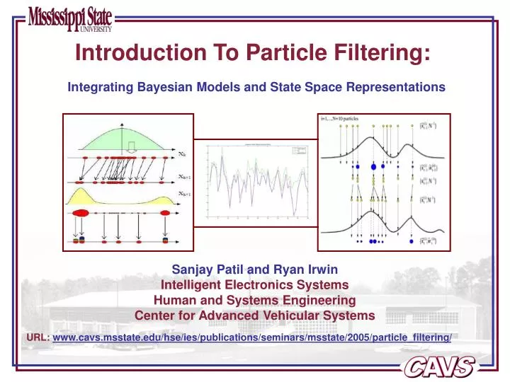
1. Introduction To Particle Filtering: Integrating Bayesian Models and State Space Representations Sanjay Patil and Ryan Irwin Intelligent Electronics Systems Human and Systems Engineering Center for Advanced Vehicular Systems URL: www.cavs.msstate.edu/hse/ies/publications/seminars/msstate/2005/particle_filtering/

2. Abstract • Conventional approaches to speech recognition use: • Gaussian mixture models to model spectral variation; • Hidden Markov models to model temporal variation. • Particle filtering: • is based on a nonlinear state space representation; • does not require Gaussian noise models; • can be used for prediction or filtering of a signal; • Approximatesthe target probability distribution (e.g. amplitude of speech signal); • also known as survival of the fittest, the condensation algorithm, and sequential Monte Carlo filters.

3. State-Space Representation General discrete-time nonlinear, non-Gaussian dynamic system  State equation  Observation (measurement) equation • Where, • Xt state vector • Yt  noisy observation vector • Ut, Vt  noise vectors • Nt  input (usually, not considered) • ft(.)  system transition function (state transition matrix) • gt(.)  measurement function (observation matrix)

4. Phase detector Se(t) Si(t) Low-pass filter, h(t) So(t) Voltage Controlled Oscillator State-space equations: • Nonlinear State Space Model – Phase Lock Loop “A device which continuously tries to track the phase of the incoming signal…” • Nonlinear feedback system • Consider a first order PLL, : AKsin( ) -

5. Hidden Markov Model and Nonlinear State-Space Model Nonlinear State-Space Model: Hidden Markov Model: • Models observations and states with non-linear and non-Gaussian functions g(.) and f(.) along with V and E being noise terms. • .Generalization of HMM • Models observations and states with transition probabilities (A), observation probabilities (B), and initial probabilities (). • Usual HMMs are modeled by first-order Markov chain. The observation probabilities can be modeled as continuous or discrete densities. The model performance improves for continuous densities as compared to discrete densities. • The calculation is based on forward-backward algorithm for evaluation (scoring)

6. Particle filter (NSSM) and CD Hidden Markov Model Nonlinear State-Space Model: CD Hidden Markov Model: Both involve Bayes rules for state computation • .Generalization of HMM • The calculation from X1, to X2 to Xn goes through a prediction and update stage with observation used to update the (predicted value) states • Use of particles to approximate the target distribution (if particle filtering is implemented). • Output – depends on prob. formulation • Can involve variable length of observations • Models Gaussian Mixtures. • The calculation is based on forward-backward algorithm for evaluation (scoring) • Finite number of means and covariance used to model the target distribution. • Output – depends on prob. formulation • Most of the times, HMMs work on a uniform length of frame (data)

7. p(X) X • Particle Filtering What is a particle? p(X)  continuous probability distribution of interest (blue)  probability distribution of interest (blue) where,  the particles  weights of the particles  the Dirac delta function  number of particles where,  approximating random measure

8. Nonlinear State-Space Model: Transition matrix Observation matrix cumbersome, intractable integrals • Nonlinear State-Space Model – particle filter • Two stages: • 1. Predict stage (using prior equation, transition matrix) • solution: • approximate representation  particle filter 2. Update stage (using filtering equation, prior, observation matrix)

9. Nonlinear State-Space Model – particle filter • Particle filter is • A method to approximate the continuous pdf • A method to sample the pdf to help compute the (intractable) integrals • Generalization of HMM. • Steps in particle filtering algorithm: (similar to Viterbi algorithm) • Generate samples to represent the initial probability • Using the prior equation, predict the next state • Using the observation, get the weights for the states computed. Predicted states (from step 2) along with the weights collectively represent the state distribution • Resample it so as to have the uniformly distributed current state omitting the least-significant representation • Continue steps 2 through 4, till all the observations are exhausted

10. Applications • Most of the applications involve tracking • Ice Hockey Game – tracking the players demo* • Ref.* Kenji Okuma, Ali Taleghani, Nando de Freitas, Jim Little and David Lowe. A Boosted Particle Filter: Multitarget Detection and Tracking. 8th European Conference on Compute Vision, ECCV 2004, Prague, CzechRepublic.http://www.cs.ubc.ca/~nando/publications.html • At IES – NSF funded project, particle filtering has been used for: • Time series estimation for speech signal^ • Ref.^M. Gabrea, “Robust adaptive Kalman Filtering-based speech enhancement algorithm,” ICASSP 2004, vol 1, pp I-301-4, May 2004. • K. Paliwal, “Estimation of noise variance from the noisy AR signal and its application in speech enhancement,” IEEE transaction on Acoustics, Speech, and Signal Processing, vol 36, no 2, pp 292-294, Feb 1988. • Speaker Verification • Speech verification algorithm based on HMM and Particle Filtering algorithm.

11. Order of Prediction Number of particles Model Estimation Feature Extraction State Predicts State Updates • Time Series Prediction Implementation : Problem statement : in presence of noise, estimate the clean speech signal. Order defines the number of previous samples used for prediction. Noise calculation is based on Modified Yule-Walker equations. yt – speech amplitude in presence of noise, xt – cleaned speech signal. part of the figure (ref): www.bioid.com/sdk/docs/About_Preprocessing.htm

12. weights update states Y(k)* = B * X(k) resampling Filtered Obsn data New Observation data • Particle filter – Detailed step by step analysis • Set-up • Speech signal is sampled at regular intervals – Observations • Idea – to filter the speech signal by particle filters • For every frame of signal, LP coefficients and noise covariance for calculated • After this is – particle filtering algorithm : Assume: order = 4, particles = 5 Five Gaussian particles samples process noise predicted state X(k) = A * X(k-1) + V(k) Observation data

13. Claimed ID Reject Accept Classifier Decision Feature Extraction Speaker Model Imposter Model Changes will be made here… • Speaker Verification Hypothesis Particle filters approximate the probability distribution of a signal If large number of particles are used, it approximates the pdf better Attempt will be made to use more Gaussian mixtures as compared to the existing system Trade-off between number of passes and number of particles

14. Pattern Recognition Applet • Java applet that gives a visual of algorithms implemented at IES • Classification of Signals • PCA - Principal Component Analysis • LDA - Linear Discrimination Analysis • SVM - Support Vector Machines • RVM - Relevance Vector Machines • Tracking of Signals • LP - Linear Prediction • KF - Kalman Filtering • PF – Particle Filtering URL: http://www.cavs.msstate.edu/hse/ies/projects/speech/software/demonstrations/applets/util/pattern_recognition/current/index.html

15. Classification Algorithms – Best Case • Data sets need to be differentiated • Classifying distinguishes between sets of data without the samples • Algorithms separate data sets with a line of discrimination • To have zero error the line of discrimination should completely separate the classes • These patterns are easy to classify

16. Classification Algorithms – Worst Case • Toroidals are not classified easily with a straight line • Error should be around 50% because half of each class is separated • A proper line of discrimination of a toroidal would be a circle enclosing only the inside set • The toroidal is not common in speech patterns

17. Classification Algorithms – Realistic Case • A more realistic case of two mixed distributions using RVM • This algorithm gives a more complex line of discrimination • More involved computation for RVM yields better results than LDA and PCA • Again, LDA, PCA, SVM, and RVM are pattern classification algorithms • More information given online in tutorials about algorithms

18. Signal Tracking Algorithms – Kalman Filter • Predicts the next state of the signal given prior information • Signals must be time based or drawn from left to right • X-axis represents time axis • Algorithms interpolate data ensuring periodic sampling • Kalman filter is shown here

19. Signal Tracking Algorithms – Particle Filter • The model has realistic noise • Gaussian noise is actually generated at each step • Noise variances and number of particles can be customized • Algorithm runs as previously described • State prediction stage • State update stage • Each step gives a collection of possible next states of signal • The collection is represented in the black particles • Mean value of particles becomes the predicted state

20. Summary • Particle filtering promises to be one of the nonlinear techniques. • More points to follow

21. References • S. Haykin and E. Moulines, "From Kalman to Particle Filters," IEEE International Conference on Acoustics, Speech, and Signal Processing, Philadelphia, Pennsylvania, USA, March 2005. • M.W. Andrews, "Learning And Inference In Nonlinear State-Space Models," Gatsby Unit for Computational Neuroscience, University College, London, U.K., December 2004. • P.M. Djuric, J.H. Kotecha, J. Zhang, Y. Huang, T. Ghirmai, M. Bugallo, and J. Miguez, "Particle Filtering," IEEE Magazine on Signal Processing, vol 20, no 5, pp. 19-38, September 2003. • N. Arulampalam, S. Maskell, N. Gordan, and T. Clapp, "Tutorial On Particle Filters For Online Nonlinear/ Non-Gaussian Bayesian Tracking," IEEE Transactions on Signal Processing, vol. 50, no. 2, pp. 174-188, February 2002. • R. van der Merve, N. de Freitas, A. Doucet, and E. Wan, "The Unscented Particle Filter," Technical Report CUED/F-INFENG/TR 380, Cambridge University Engineering Department, Cambridge University, U.K., August 2000. • S. Gannot, and M. Moonen, "On The Application Of The Unscented Kalman Filter To Speech Processing," International Workshop on Acoustic Echo and Noise, Kyoto, Japan, pp 27-30, September 2003. • J.P. Norton, and G.V. Veres, "Improvement Of The Particle Filter By Better Choice Of The Predicted Sample Set," 15th IFAC Triennial World Congress, Barcelona, Spain, July 2002. • J. Vermaak, C. Andrieu, A. Doucet, and S.J. Godsill, "Particle Methods For Bayesian Modeling And Enhancement Of Speech Signals," IEEE Transaction on Speech and Audio Processing, vol 10, no. 3, pp 173-185, March 2002. • M. Gabrea, “Robust Adaptive Kalman Filtering-based Speech Enhancement Algorithm,” ICASSP 2004, vol 1, pp. I-301-I-304, May 2004. • K. Paliwal, :Estiamtion og noise variance from the noisy AR signal and its application in speech enhancement,” IEEE transaction on Acoustics, Speech, and Signal Processing, vol 36, no 2, pp 292-294, Feb 1988.

22. References (for PLL): • Modern Digital and Analog Communication Systems B.P. Lathi, Oxford University Press, Second Edition. • Andrew J. Viterbi, “Phase-Locked Loop Dynamics in the presence of noise by Fokker-Planck Techniques”, Proceedings of the IEEE, 1963.

23. References (HMM and particle): • M. Andrews, “Learning and Inference in Nonlinear State- Space Models,” (in preparation). • V. Digalakis, J. Rohlicek, and M. Ostendorf, “,” IEEE transactions on Speech and Audio Processing, vol 1, no 4, October 1993, pp 431-434.

24. Proof for the predict stage equation: Observations independent given the states

25. State-Space Equation and State-Variable Equation State-Space Equation: State-Variable Equation: Both involve matrix algebra, carry same names, similar meanings • Parameters required are: • F, H, G, X0, p(X0), noise statistics, covariance terms, • Vk and Ek are noise terms • The calculation from X1, to X2 to Xn goes through a prediction and update stage with observation used to update the (predicted value) states. • Output term: Xk (hidden / unknown) • Parameters required are: • F, H, G, X0, U0(input) • The calculation from X1, to X2 to Xn goes through only one stage. Idea is to find observations Yk. • Output term: Yk (output / not hidden)