Download
1 / 18
180 likes | 336 Views
Variational Assimilation of HF Radar Surface Currents into the Coastal Ocean Circulation Model off Oregon. Peng Yu in collaboration with Alexander Kurapov, Gary Egbert, John S. Allen, P. Michael Kosro College of Oceanic and Atmospheric Sciences Oregon State University. Supported by ONR.

E N D
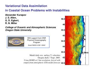
Variational Assimilation of HF Radar Surface Currents into the Coastal Ocean Circulation Model off Oregon Peng Yu in collaboration with Alexander Kurapov, Gary Egbert, John S. Allen, P. Michael Kosro College of Oceanic and Atmospheric Sciences Oregon State University Supported by ONR
Complicated dynamics on the shelf in the • coastal transition zone (CTZ): • Strong upwelling season • Modeling sensitive to many factors (model resolution, horizontal eddy viscosity, bathymetry, boundary conditions, forcing) • Use data assimilation to improve prediction, forecasting, and scientific understanding of shelf and CTZ flows 6-km, visc=10 m2/s Model details: Regional Ocean Modeling System (ROMS) - 6km horizontal resolution and 15 vertical level - NOOA -NAM wind & heat flux - NCOM-CCS boundary conditions (Shulman et al., NRL) (shown: SST Jul. 20, 2008)
Summer 2008: available observations Bathymetric contours: 1000 and 200 m) • - HF radar surface velocities (daily maps, provided by PM Kosro, OSU) • Combination of several standard and long-range radar provides time-series info about shelf, slope and CTZ flows • SSH along track altimetry (Jason, Envisat) • satellite SST maps (D. Folley, NOAA CoastWatch) • gliders (T and S sections, once every 3 days, J Barth and R. K. Shearman, OSU) – 3D information How does each of these data types contribute to data assimilation?
Variational (representer-based) data assimilation • in a series of 3-day time windows, June 1– July 30, 2008: • In each window, • correct initial conditions (use tangent linear &adjoint codes AVRORA, developed at OSU, Kurapov et al., Dyn. Atm. Oceans, 2009) • run the nonlinear ROMS for 6 days (analysis + forecast) assim (TL&ADJ AVRORA) forecast (NL ROMS) forecast analysis prior
The representer-based DA system the representer function
Indirect method (Egbert et al. 1994; Chua and Bennett, 2001) Forecast model • Indirect method is computationally more efficient • Conjugate Gradient method • Preconditioned Conjugate Gradient Adjoint model Tangent Linear model Task Parallel …. Precondition …. Conjugate Gradient (5-10 steps) (Egbert, 1997)
Initial Condition Error Covariance (Dynamically balanced): multivariate u, v, SSH, T, S – geostrophy, thermal-wind Implement the balance operator A (Weaver et al. 2005): Adj solution at ini time univariate covariance for mutually uncorrelated fields s • A: • Uncorrelated fields: error in T and depth-integrated transport (uH, vH) • S (using constant T-S relationships) • horizontal density gradients • vertical shear in u, v (thermal wind balance) • SSH (2nd order ellipitic eqn.) • u, v (surface current in geostrophic balance with SSH)
Initial test with one 3-day assimilation window (balanced covariances better in SST forecast) Surface Velocity SST (not assimilated) RMSE Correlation Analysis Forecast Analysis Forecast SST data provided by D. Foley, NOAA CoastWatch
Same experiment: extend the forecast to 15days Surface Velocity SST (not assimilated) RMSE Balanced better Correlation Analysis Analysis Forecast Forecast SST RMSE and correlation are improved for 15 days, after the 1st assimilation cycle
60-day assimilation (June 1-July 30, 2008; 20 assimilation windows): Both Surface velocity and SST are improved Surface Velocity SST (not assimilated) RMSE Correlation
Model data comparison: Surface currents (assimilated) and SST (not assimilated) Assimilation of HF radar surface currents improves the geometry of the upwelling SST front
The time-averaged sea surface currents field: more uniform cross-shore transport than in prior Observation Prior Forecast Analysis
The mean and variance ellipses of the model-data difference Mean: Obs-Forecast Mean: Obs-Analysis Mean: Obs-Prior Variances Variances Variances
Assimilation of HFR data improves SSH, compared to along-track altimetry (not assimilated) in the area covered by the HF Radar Verification SSH, prior, HF radar velocity assimilation Data coverage
Cont. (another pass) Verification SSH, prior, HF radar velocity assimilation Data coverage
Comparison against Hydrographic data Analysis (balanced) Analysis (Imbalanced) Observation Prior -The assimilation of the HF Radar surface currents data improves the density structure in the hydrographic sections south of Cape Blanco in the separation zone NH CC RR Data provided by Bill Peterson and Jay Peterson)
Summary • The representer-based data assimilation system improves the forecast of the model variables (e.g. SST, surface currents, SSH, density) • The assimilation of unique set of long-range HF radar observations has a positive impact on the area of the shelf, slope and part of the open ocean • Assimilation of the HF Radar radial component might be advantageous • A combination of different types of observations is being pursued