Download
1 / 57
580 likes | 1.15k Views
Chapter 7 Hypothesis Testing. 7-1 Overview 7-2 Basics of Hypothesis Testing 7-3 Testing a Claim About a Proportion 7-5 Testing a Claim About a Mean: Not Known 7-6 Testing a Claim About a Standard Deviation or Variance. Chapter 7 Hypothesis Testing. Definition Hypothesis

E N D
7-1 Overview 7-2 Basics of Hypothesis Testing 7-3 Testing a Claim About a Proportion 7-5 Testing a Claim About a Mean: Not Known 7-6 Testing a Claim About a Standard Deviation or Variance Chapter 7Hypothesis Testing
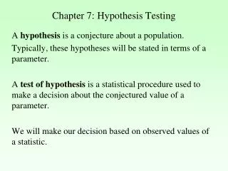
Definition Hypothesis in statistics, is a claim or statement about a property of a population 7-1 Overview
Definition Hypothesis Test is a standard procedure for testing a claim about a property of a population 7-1 Overview
If, under a given assumption, the probability of a particular observed event is exceptionally small, we conclude that the assumption is probably not correct. Rare Event Rule for Inferential Statistics
Example: ProCare Industries, Ltd., once provided a product called “Gender Choice,” which, according to advertising claims, allowed couples to “increase your chances of having a boy up to 85%, a girl up to 80%.” Suppose we conduct an experiment with 100 couples who want to have baby girls, and they all follow the Gender Choice directions in the pink package. For the purpose of testing the claim of an increased likelihood for girls, we will assume that Gender Choice has no effect. Using common sense and no formal statistical methods, what should we conclude about the assumption of no effect from Gender Choice if 100 couples using Gender Choice have 100 babies consisting of a) 52 girls?; b) 97 girls?
Example: ProCare Industries, Ltd.: Part a) a) We normally expect around 50 girls in 100 births. The results of 52 girls is close to 50, so we should not conclude that the Gender Choice product is effective. If the 100 couples used no special method of gender selection, the result of 52 girls could easily occur by chance. The assumption of no effect from Gender Choice appears to be correct. There isn’t sufficient evidence to say that Gender Choice is effective.
Example: ProCare Industries, Ltd.: Part b) b) The result of 97 girls in 100 births is extremely unlikely to occur by chance. We could explain the occurrence of 97 girls in one of two ways: Either an extremely rare event has occurred by chance, or Gender Choice is effective. The extremely low probability of getting 97 girls is strong evidence against the assumption that Gender Choice has no effect. It does appear to be effective.
7-2 Basics of Hypothesis Testing
Given a claim, identify the null hypothesis, and the alternative hypothesis, and express them both in symbolic form. Given a claim and sample data, calculate the value of the test statistic. Given a significance level, identify the critical value(s). Given a value of the test statistic, identify the P-value. State the conclusion of a hypothesis test in simple, non-technical terms. Identify the type I and type II errors that could be made when testing a given claim. 7-2 Section Objectives
Example:Let’s again refer to the Gender Choice product that was once distributed by ProCare Industries. ProCare Industries claimed that couple using the pink packages of Gender Choice would have girls at a rate that is greater than 50% or 0.5. Let’s again consider an experiment whereby 100 couples use Gender Choice in an attempt to have a baby girl; let’s assume that the 100 babies include exactly 52 girls, and let’s formalize some of the analysis. Under normal circumstances the proportion of girls is 0.5, so a claim that Gender Choice is effective can be expressed as p > 0.5. Using a normal distribution as an approximation to the binomial distribution, we find P(52 or more girls in 100 births) = 0.3821. continued
Example:Let’s again refer to the Gender Choice product that was once distributed by ProCare Industries. ProCare Industries claimed that couple using the pink packages of Gender Choice would have girls at a rate that is greater than 50% or 0.5. Let’s again consider an experiment whereby 100 couples use Gender Choice in an attempt to have a baby girl; let’s assume that the 100 babies include exactly 52 girls, and let’s formalize some of the analysis. Figure 7-1 shows that with a probability of 0.5, the outcome of 52 girls in 100 births is not unusual. continued
We do not reject random chance as a reasonable explanation. We conclude that the proportion of girls born to couples using Gender Choice is not significantly greater than the number that we would expect by random chance. Figure 7-1
Claim: For couples using Gender Choice, the proportion of girls is p > 0.5. Working assumption: The proportion of girls is p = 0.5 (with no effect from Gender Choice). The sample resulted in 52 girls among 100 births, so the sample proportion is p = 52/100 = 0.52. Key Points ˆ
Assuming that p = 0.5, we use a normal distribution as an approximation to the binomial distribution to find that P(at least 52 girls in 100 births) = 0.3821. There are two possible explanation for the result of 52 girls in 100 births: Either a random chance event (with probability 0.3821) has occurred, or the proportion of girls born to couples using Gender Choice is greater than 0.5. There isn’t sufficient evidence to support Gender Choice’s claim. Key Points
Statement about value of population parameter that is equal to some claimed value H0: p = 0.5 H0: = 98.6 H0: = 15 Test the Null Hypothesis directly Reject H0 or fail to reject H0 Null Hypothesis: H0
the statement that the parameter has a value that somehow differs from the null Must be true if H0 is false , <, > Alternative Hypothesis: H1
H0: Must contain equality H1: Will contain , <, > Claim: Using math symbols
Note about Identifying H0 and H1 Figure 7-2
If you are conducting a study and want to use a hypothesis test to support your claim, the claim must be worded so that it becomes the alternative hypothesis. This means your claim must be expressed using only , <, > Note about Forming Your Own Claims (Hypotheses)
z = p - p Test statistic for proportions pq n Test Statistic The test statistic is a value computed from the sample data, and it is used in making the decision about the rejection of the null hypothesis.
x - µx Test statistic for mean z= n Test Statistic The test statistic is a value computed from the sample data, and it is used in making the decision about the rejection of the null hypothesis.
x - µx Test statistic for mean t= s n Test Statistic The test statistic is a value computed from the sample data, and it is used in making the decision about the rejection of the null hypothesis.
(n – 1)s2 2= 2 Test Statistic The test statistic is a value computed from the sample data, and it is used in making the decision about the rejection of the null hypothesis. Test statistic for standard deviation
Example:A survey of n = 880 randomly selected adult drivers showed that 56%(or p = 0.56) of those respondents admitted to running red lights. Find the value of the test statistic for the claim that the majority of all adult drivers admit to running red lights. (In Section 7-3 we will see that there are assumptions that must be verified. For this example, assume that the required assumptions are satisfied and focus on finding the indicated test statistic.) ˆ
z = p – p = 0.56 - 0.5 = 3.56 pq (0.5)(0.5) n 880 Solution:The preceding example showed that the given claim results in the following null and alternative hypotheses: H0: p = 0.5 and H1: p > 0.5. Because we work under the assumption that the null hypothesis is true with p = 0.5, we get the following test statistic:
Interpretation:We know from previous chapters that a z score of 3.56 is exceptionally large. It appears that in addition to being “more than half,” the sample result of 56% is significantly more than 50%. See Figure 7-3 where we show that the sample proportion of 0.56 (from 56%) does fall within the range of values considered to be significant because they are so far above 0.5 that they are not likely to occur by chance (assuming that the population proportion is p = 0.5).
Set of all values of the test statistic that would cause a rejection of the null hypothesis CriticalRegion (or Rejection Region)
Set of all values of the test statistic that would cause a rejection of the null hypothesis Critical Region Critical Region
Set of all values of the test statistic that would cause a rejection of the null hypothesis Critical Region Critical Region
Set of all values of the test statistic that would cause a rejection of the null hypothesis Critical Region Critical Regions
denoted by the probability that the test statistic will fall in the critical region when the null hypothesis is actually true. same introduced in Section 6-2. common choices are 0.05, 0.01, and 0.10 Significance Level
Any value that separates the critical region (where we reject the null hypothesis) from the values of the test statistic that do not lead to a rejection of the null hypothesis Critical Value
Any value that separates the critical region (where we reject the null hypothesis) from the values of the test statistic that do not lead to a rejection of the null hypothesis Critical Value Critical Value ( z score )
Any value that separates the critical region (where we reject the null hypothesis) from the values of the test statistic that do not lead to a rejection of the null hypothesis Critical Value Reject H0 Fail to reject H0 Critical Value ( z score )
Two-tailed,Right-tailed,Left-tailed Tests The tails in a distribution are the extreme regions bounded by critical values.
H0: = H1: Means less than or greater than Values that differ significantly from H0 Two-tailed Test is divided equally between the two tails of the critical region
H0: = H1: > Right-tailed Test Points Right Values that differ significantly from Ho
H0: = H1: < Left-tailed Test Points Left Values that differ significantly from Ho
P-Value The P-value (or p-value or probability value) is the probability of getting a value of the test statistic that is at leastas extreme as the one representing the sample data, assuming that the null hypothesis is true. The null hypothesis is rejected if the P-value is very small, such as 0.05 or less.
Example:Finding P-values Figure 7-6
always test the null hypothesis 1. Reject the H0 2. Fail to reject the H0 Conclusions in Hypothesis Testing
Decision Criterion Traditional method: Reject H0 if the test statistic falls within the critical region. Fail torejectH0if the test statistic does not fall within the critical region.
Decision Criterion P-value method: Reject H0 if P-value (where is the significance level, such as 0.05). Fail torejectH0if P-value > .
Decision Criterion Another option: Instead of using a significance level such as 0.05, simply identify the P-value and leave the decision to the reader.
Decision Criterion Confidence Intervals: Because a confidence interval estimate of a population parameter contains the likely values of that parameter, reject a claim that the population parameter has a value that is not included in the confidence interval.
Wording of Final Conclusion Figure 7-7