Download
1 / 65
760 likes | 1.25k Views
Interferometric Synthetic-Aperture Radar (InSAR) and Applications. Chris Allen (callen@eecs.ku.edu) Course website URL www.cresis.ku.edu/~callen/826/EECS826.htm. Outline. Syllabus Instructor information, course description, prerequisites Textbook, reference books, grading, course outline

E N D
Interferometric Synthetic-Aperture Radar (InSAR) and Applications Chris Allen (callen@eecs.ku.edu) Course website URL www.cresis.ku.edu/~callen/826/EECS826.htm
Outline • Syllabus • Instructor information, course description, prerequisites • Textbook, reference books, grading, course outline • Preliminary schedule • Introductions • What to expect • First assignment • Radar fundamentals • Active RF/microwave remote sensing • Electromagnetic issues • Antennas • Resolution (spatial, range)
Syllabus • Prof. Chris Allen • Ph.D. in Electrical Engineering from KU 1984 • 10 years industry experience Sandia National Labs, Albuquerque, NM AlliedSignal, Kansas City Plant, Kansas City, MO • Phone: 785-864-3017 • Email: callen@eecs.ku.edu • Office: 321 Nichols Hall • Office hours: Tuesdays and Thursdays 2:00 to 2:30 p.m. and 3:45 to 4:30 p.m. • Course description • Description and analysis of processing data from synthetic-aperture radars and interferometric synthetic-aperture radars. Topics covered include SAR basics and signal properties, range and azimuth compression, signal processing algorithms, interferometry and coregistration.
Syllabus • Prerequisites • Introductory course on radar systems (e.g., EECS 725) • Introductory course on radar signal processing (e.g., EECS 744) • Textbook • Processing of SAR Data by A. HeinSpringer, 2004, ISBN 3540050434
Syllabus • Reference books • Synthetic Aperture Radar Processingby G. Franschetti and R. LanariCRC Press, 1999, ISBN 0849378990 • Digital Processing of Synthetic Aperture Radar Databy I. Cumming and F. WongArtech House, 2005, ISBN 1580530583 • Spotlight-Mode Synthetic Aperture RadarC. Jakowatz, et al,Springer, 1996, ISBN 0792396774 • Synthetic Aperture Radar: Systems and Signal ProcessingJ. Curlander and R. McDonoughWiley, 1991, ISBN 047185770X
Grades and course policies • The following factors will be used to arrive at the final course grade: • Homework, quizzes, and class participation 40 % Research project 20 % Final exam 40 % • Grades will be assigned to the following scale: • A 90 - 100 % B 80 - 89 % C 70 - 79 % D 60 - 69 % F < 60 % • These are guaranteed maximum scales and may be revised downward at the instructor's discretion. • Read the policies regarding homework, exams, ethics, and plagiarism.
Preliminary schedule • Course Outline (subject to change) • SAR system overview and signal properties 1 weeks(data recording, nonideal motion, layover and shadowing, moving targets) • SAR radar range equation and associated geometries 2 weeks(side-looking, squint, and spotlight modes) • SAR signal processing 3 weeks(range and azimuth compression, range migration, autofocus) • SAR signal processing algorithms 2 weeks(range-Doppler, scaling, omega-k) • Interferometry 6 weeks(registration, decorrelation, phase unwrapping, implementation, terrain mapping, surface velocity mapping, change detection, single-pass vs. multi-pass) • Class Meeting Schedule • January: 15, 20, 22, 27, 29 • February: 3, 5, (10th to 12th NSF Site Visit), 17, 19, 24, 26 • March: 3, 5, 10, 12, (17th to 19th Spring Break), 24, 26, 31 • April: 2, 7, 9, 14, 16, 21, 23, 28, 30 • May: 5, 7 • Final exam scheduled for Friday, May 15, 1:30 to 4:00 PM
Introductions • Name • Major • Specialty • What you hope to get from of this experience • (Not asking what grade you are aiming for )
What to expect • Course is being webcast, therefore … • Most presentation material will be in PowerPoint format • Presentations will be recorded and archived (for duration of semester) • Student interaction is encouraged • Students must activate microphone before speaking • Please disable microphone when finished • Homework assignments will be posted on website • Electronic homework submission logistics to be worked out • We may have guest lecturers later in the semester • To break the monotony, we’ll try to take a couple of 2-minute breaks during each session (roughly every 15 to 20 min)
Your first assignment • Send me an email (from the account you check most often) • To: callen@eecs.ku.edu • Subject line: Your name – EECS 826 • Tell me a little about yourself • Attach your ARTS form (or equivalent) • ARTS: Academic Requirements Tracking System • Its basically an unofficial academic record • I use this to get a sense of what academic experiences you’ve had
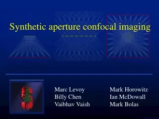
SAR image of Los Angeles area SEASAT Synthetic Aperture Radarf: 1.3 GHz PTX: 1 kWant: 10.8 x 2.2 m B: 19 MHzx = y = 25 m pol: HHorbit: 795 km DR: 110 Mb/s
SEASAT suffered a massive electrical short in one of the slip ring assemblies used to connect the rotating solar arrays to the power subsystem.
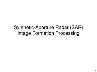
SAR image of Gibraltar ERS-1 Synthetic Aperture Radarf: 5.3 GHz PTX: 4.8 kWant: 10 m x 1 m B: 15.5 MHzx = y = 30 m fs: 19 MSa/sorbit: 780 km DR: 105 Mb/s Nonlinear internal waves propagating eastwards and oil slicks can be seen.
Radar fundamentals (review) • ERS-1 Synthetic Aperture Radar • Radar center frequency, f: 5.3 GHz • C-band, = c/f = 5.7 cm c = 3 x 10⁸ m/s • Antenna dimensions, ant: 10 m x 1 m (width x height) • Approx. beamwidth, /antenna dimension • az 0.057 m/10 m = 5.7 mrad or 0.32° • el 0.057 m/1 m = 57 mrad or 3.2° • Antenna gain, G 4/(az el) • G(dBi) = 10 log10(G) dBi is dB relative to isotropic antenna • G = 4/(0.057 x 0.0057) = 38700 or 46 dBi • Minimum along-track resolution, ymin = ℓ/2 ℓ is antenna’s along-track dimension • ℓ = 10 m, ymin = 5 m, y = 30 m > ymin • Bandwidth, B: 15.5 MHz • Range resolution (slant range, cross-track), r = c/2B • r = c/(2 x 15.5 MHz) = 9.7 m • Ground resolution (cross-track), x = r /sin is the incidence angle • Pulse duration, : 37.1 s • Pulse compression ratio, B = 575 (28 dB) B(dB) = 10 log10(B) • Blind range c/2 = 5.6 km
Radar fundamentals (review) • ERS-1 Synthetic Aperture Radar • Sampling frequency, fs: 19 MSa/s, 5 b/sample, I/Q • Nyquist requires fs≥ 15.5 MSa/s • fs = 1.23 Nyquist rate (23% oversampling) • Orbit altitude, h: 780 km • Orbital velocity, v, for Earth, = 398,600 km3/s2 • Ground velocity, vg, Re = 6378.145 km • v = 7.46 km/s, vg = 6.65 km/s • Minimum pulse-repetition frequency, PRFmin = 2v/ℓ • PRFmin = 2(7460)/10 = 1490 Hz • 1720 Hz ≥ PRF ≥ 1640 Hz (from ERS specs) • Look angle, : 23° • sin = (1 + h/Re) sin • = 26° • Ground resolution, x = r /sin • x = 22 m
Radar fundamentals (review) • ERS-1 Synthetic Aperture Radar • Ground swath width, Wgr: 100 km • Slant swath width, Wr = Wgr sin • Wr = 43.8 km • Echo duration from swath, s = + 2 Wr/c • s = 37.1 s + 292 s = 329.1 s • Data rate, DR: 105 Mb/s • Samples/echo = 329.1 s x 19 MSa/s = 6250 Samples/echo • Sample rate = PRF x Samples/echo • Sample rate = 1640 x 6300 = 10.3 MSa/s • Data rate = Sample rate x bits/sample = 10.3 MSa/s x 10 bits/Sa = 103 Mb/s
Ka-band, 4″ resolutionHelicopter and plane static display f: 35 GHz
Radar fundamentals (review) • Radar range equation, received signal power, and signal-to-noise ratio • For a monostatic radar system and a point target • Where • Pt is the transmitted signal power, WPr is the power intercepted by the receiver, WG is the gain of the antenna in the direction of the targetR is the range from the antenna to the scatterer, m is the target’s radar scattering cross section (RCS), m2 is the wavelength of the radar signal, m
Radar fundamentals (review) • Receiver noise power, PN • k is Boltzmann’s constant (1.38 10-23 J K-1) • T0 is the absolute temperature (290 K) • B is receiver bandwidth, Hz • F is receiver noise figure • Signal-to-noise ratio (SNR) is • may be expressed in decibels
Radar fundamentals (review) • Example: Sandia Lynx SAR • Radar center frequency, f = 16 GHz • Transmit power, PT = 320 W (55.1 dBm) dBm: dB relative to 1 mW • Slant range resolution, r= 0.3 m (1 ft) • Receiver noise figure, FREC = 2.8 (F = 4.5 dB) • Antenna beamwidths, 3.2° x 7° • Range to target, R = 30 km (18.6 miles) • Target RCS, = 0.001 m2(-30 dBsm) = ° x y • Find the Pr , PN , and the SNR • First derive some related radar parameters Wavelength, = c/f = 0.01875 m Antenna gain, G 4/(az el) G = 1840 or 32.6 dBi Bandwidth, B = c/2r B = 500 MHz
Radar range equation example • Find Pr • Solve in dB • Pr(dBm) = Pt(dBm) + 2G(dBi) + 2 (dB) + (dBsm) – 3 4(dB) – 4 R(dB) • Pt(dBm) = 55.1 G(dBi) = 32.6 (dB) = -17.3 (dBsm) = -30 • 4(dB) = 11 R(dB) = 44.8 • Pr(dBm) = -156.3 dBm or 2.3 10-19 W (0.23 aW) • Find PN • Solve in dB • PN(dBm) = kT0(dBm) + B(dB) + F(dB) • kT0(dBm) = -174 B(dB) = 87 F(dB) = 4.5 • PN(dBm) = -82.5 dBm or 5.6 pW • Find SNR • SNR = – 156.3 – (– 82.5) = -73.7 dB or 4.3 10-8
Radar fundamentals (review) • Signal processing improves SNR • Pulse compression gain, B • Assuming = 20 s yields a 40-dB pulse compression gain • Coherent integration improves SNR by N • N is the number of integrations • N = synthetic-aperture length * PRF / velocity • Synthetic-aperture length, L = az R, L = 1675 m • Assume velocity = 36 m/s (Predator UAV cruise speed is 130 km/h ) • Assuming a 1-kHz PRF • N = 46500 or 46-dB improvement • Therefore the SNR from a -30-dBsm target is 12.3 dB • Many measurements require SNR > 10 dB
Airborne SAR block diagram New terminology:Magnitude imagesMagnitude and Phase ImagesPhase HistoriesMotion compensation (MoComp)Autofocus Timing and ControlInertial measurement unit (IMU)GimbalChirp (Linear FM waveform)Digital-Waveform Synthesizer
Airborne SAR real-time IFP block diagram Image-Formation Processor New terminology:Presum (a.k.a. coherent integration)Corner-turning memory (CTM)Window Function Focus and Correction VectorsRange Migration and Range WalkFast Fourier transform (FFT)Chirp-z transform (CZT)
Radar response to extended targets • The preceding development considered point target with a simple RCS, . • The point-target case enables simplifying assumptions in the development. • Gain and range are treated as constants • Consider the case of extended targets including surfaces and volumes. • The backscattering characteristics of a surface are represented by the scattering coefficient, , • where A is the illuminated area.
Factors affecting backscatter • The backscattering characteristics of a surface are represented by the scattering coefficient, • For surface scattering, several factors affect • Dielectric contrast Large contrast at boundary produces large reflection coefficient Air (r = 1), Ice (r ~ 3.2), (Rock (4 r 9), Soil (3 r 10), Vegetation (2 r 15), Water (~ 80), Metal (r ) • Surface roughness (measured relative to ) RMS height and correlation length used to characterize roughness • Incidence angle, () • Surface slope Skews the () relationship • Polarization VV HH» HV VH
Backscatter from bare soil Note: At 1.1 GHz, = 27.3 cm
Detecting flooded lands • Combination of water surface and vertical tree trucks forms natural dihedral with enhanced backscatter.
Doppler shifts and radial velocity • The signal from a target may be written as • c = 2fc • and the relative phase of the received signal, • A target moving relative to the radar produces a changing phase (i.e., a frequency shift) known as the Doppler frequency,fD • where vr is the radial component of the relative velocity. • The Doppler frequency can be positive or negative with a positive shift corresponding to target moving toward the radar.
Doppler shifts and radial velocity • The received signal frequency will be • Example • Consider a police radar with a operating frequency, fo, of 10 GHz. ( = 0.03 m) • It observes an approaching car traveling at 70 mph (31.3 m/s) down the highway. (v = -31.3 m/s) • The frequency of the received signal will be • fo – 2v/ = fo+ 2.086 kHz or 10,000,002,086 Hz • Another car is moving away down the highway traveling at 55 mph (+24.6 m/s). The frequency of the received signal will be • fo – 2v/ = fo– 1.64 kHz or 9,999,998,360 Hz
Doppler shifts and radial velocity ^ uR = u cos(q) fD = 2 u cos(q) / l • Given the position, P, and velocity, u, both the radar and the target, the resulting Doppler frequency can be determined • The ability to resolve targets based on their Doppler shifts depends on the processed bandwidth, B, that is inversely related to the observation (or integration) time, T Instantaneous position and velocity Relative velocity, u Radial velocity component
Pulse repetition frequencies (PRFs) The lower limit for PRFs is driven byDoppler ambiguities
Doppler ambiguities • To unambiguously reconstruct a waveform, the Nyquist-Shannon sampling theorem (developed and refined from the 1920s to 1950s at Bell Labs) states that exact reconstruction of a continuous-time baseband signal from its samples is possible if the signal is bandlimited and the sampling frequency is greater than twice the signal bandwidth. • Application to radar means that the pulse-repetition frequency (PRF) must be at least twice the Doppler bandwidth. For side-looking SAR (centered about 0 Doppler), the PRF must be twice the highest Doppler shift. • For the case where the Doppler frequency shift will be 250 Hz (a 500-Hz Doppler bandwidth), the PRF must be at least 500 Hz. • [The Nyquist-Shannon theorem also has application to signal digitization in the analog-to-digital converter (ADC) requiring that the ADC sampling frequency be at least twice the waveform bandwidth.]
PRF constraints • Recapping what we’ve seen— • The lower PRF limit is determined by Doppler ambiguities • The upper PRF limit is determined by the range ambiguities • Eclipsing • Furthermore, for systems that do not support receiving while transmitting, various forbidden PRFs will exist that will eclipse the receive intervals with transmission pulses, which leads to • where Tnear and Tfar refer to signal arrival times for near and far targets, is the transmit pulse duration, and N represents whole numbers (1, 2, 3, …) corresponding to pulses
Spherical Earth calculations • Spherical Earth geometry calculations • ReEarth’s average radius (6378.145 km) • h orbit altitude above sea level (km) • core angle • R radar range • look angle • i incidence angle
Spherical Earth calculations • Satellite orbital velocity calculations (for circular orbits) • ReEarth’s average radius (6378.145 km) • h orbit altitude above sea level (km) • v satellite velocity • vg satellite ground velocity • standard gravitational parameter (398,600 km3/s2 for Earth)
Spherical Earth calculations • Swath width geometry calculations • ReEarth’s average radius (6378.145 km) • Rn range to swath’s near edge • Rf range to swath’s far edge • Wgr swath width on ground • Wr slant range swath width • n core angle to swath’s near edge • f core angle to swath’s far edge • i,m incidence angle at mid-swath