Download
1 / 18
190 likes | 323 Views
Interval packing problem. Multicommodity demand flow in a line. Jian Li Sep. 2005. Interval packing problem. Input:

E N D
Interval packing problem Multicommodity demand flow in a line Jian Li Sep. 2005
Interval packing problem • Input: • 1) A set I of n intervals, I1, I2, ..., In, with each Ii = [li, ri] and having a THICKNESS (or HEIGHT) hi, such that li and ri are all integers in {1,2, ..., n} and hi is an integer > 0 • 2) n-1 CAPACITY constraints ci, with each ci located at the point pi = (i + 1/2, 0) on the x-axis, for every i = 1,2, ..., n-1, such that each ci is an integer > 0. We may call each pi a thickness constrained point • Output: • The MAXIMUM NUMBER of intervals in I such that at each thickness constrained point pi = (i + 1/2, 0), the sum of thickness values of all output intervals that contain pi is less then ci.
In fact, it is a special case of the multicommodity demand flow problem
Multicommodity demand flow problem • T=(V,E,u) be a capacitated network, where each edge capacity ue is an integer. • A number of demand vertices pairs (si,ti) with demand value di and profit wi • GOAL: simultaneously route the demand flow without violating the capacity constraints and maximize the profit. • NOTE: di must be fully satisfied to obtain a profit wi
Interval packing problem can be modeled as multicommodity flow problem in a line.
LP formulation max i wixi i:e2 path(i)dixi· ue xi=0,1
Some special case • All capacities are one. • All demand are one. • The problem is exactly to compute a independent set in a interval graph, which is in P.
Algorithm: • Sort intervals according their left endpoints. • Use the reverse order to greedy construct the independent set. (reverse perfect elimination order)
Some special case. • the problem can be formulated as the following min-cost flow problems. • There are n vertice, namely v1,v2,…..,vn, and arcs from vi to v(i+1) with capacity ui and cost zero and arc from vn to v1 with capacity +infinity and cost zero. • For every interval Ii, there is a arc from v(ri) to v(li) with capacity di and cost -1/di(we call it back-arc).
Some special case • However, the min cost circulation may not give the correct answer, because in the original problem only in case that the back-arc are saturated(flow=capacity) can incur a cost 1. So we can treat it as the relax of the original problem. In fact it solve the relaxed LP of the original problem. • Moreover, if all di is one, then this special case can be solved optimally in polytime.
Some special case • if the number of intervals passing pi is bounded( less than a constant C), then we can solve the problem optimally by standard dynamic programming technique.
Small and Large demand • Bottleneck capacity b(f): the smallest capacity edge on Path(f) • -large demand: d(f)¸ b(f) • Otherwise ,-small
Bounding large demand • Lemma: • If dmax· umin (a wild assumption)in a feasible solution, the number of -large demands that cross any edge is at most 2(1/2) • So, we can use DP to solve the case with only large task optimally.
Bounding large demand • Proof of the lemma: • Fix a feasible solution S, consider an edge e. • Let Se be the set of all -large demand cross e. • Se=Sl[ Sr, where Sl is the set where its bottleneck is to the left of e(including e), and Sr otherwise. Sr Sl e
Bounding large demand • Proof Cont. • We can show Sl<=1/2 (similar for Sr) • Let A be the set of bottleneck edge for Sl. Let e’ be the rightmost one in A. Suppose e’ is the bottleneck edge for demand Ij, thus dj> c(e’). But all demands in Sl pass through e’(since e’ is rightmost one). But each demand Ik is -large. dk¸ bk¸ cmin. • cminSl· c(e’), thus • Sl· |c(e’)/cmin| · |di/2 cmin| · 1/2 \QED
Suppose we have a -approximation algorithm for the case where only small demands exist. • Then we choose the larger one from the optimal solution for large demand and approximation solution for small demand • We get 2 approximation for original problem OPT<=OPTlarge+OPTsmall<=SOLlarge+ SOLsmall <=2max{SOLlarge+ SOLsmall} <= 2 max{SOLlarge+ SOLsmall}
Dealing with Small demands • Randomized rounding: G.Calineascu et IPCO2002 for uniform capacity. (1+e)-approx. A.Chakrabarti et APPROX2002 for general case. O(1)-approx. • Packing integer program C.Chekuri et ICALP2003 for general case. (1+e)-approx.