Download
1 / 33
350 likes | 586 Views
Simulating the Production of Ethanol. Student Name 1 Student Name 2 Student Name 3. Overview. Introduction to Production Simulation Results Conclusion. Ethanol Production. Fermenter. Fermentation Reaction. Zymase. 2. +. + Heat. Glucose. Ethanol. Carbon Dioxide. Chemical Equation.

E N D
Simulating the Production of Ethanol Student Name 1 Student Name 2 Student Name 3
Overview • Introduction to Production • Simulation • Results • Conclusion
Ethanol Production Fermenter
Zymase 2 + + Heat Glucose Ethanol Carbon Dioxide Chemical Equation
Developing the System • Based on Mass Balances • And Energy Balance
Temperature Dependency • Reaction Rate • Heat
CO2 CGin, CEin, Tin, Fin Yeast CG, CE, T, F Q V, ρ, CP Reactor
Methods of Solution • MATLAB • Simulink • Laplace Transform using Maple
MATLAB Code: Steady State %steady state function conc=ustank(t,solution) global Tin V Fin Fout CEin Cgin B rho Cp T=solution(1); Cg=solution(2); CE=solution(3); rate=Cg*10^3*exp(-50/T) Cgin=150 conc(1,1)=(Tin*Fin*Cp*rho-T*Fout*rho*Cp+B*rate)/(V*rho*Cp); conc(2,1)=(Cgin*Fin-Cg*Fout-(rate))/V; conc(3,1)=(CEin*Fin-CE*Fout+0.5*rate)/V;
Linear Approximations • Taylor Series Expansion • Approximate Methods:
Laplace Transform E’(t) = -0.57e-1*exp(-0.14e-2*t)*cos(0.39e-4*t) +0.22e-1*exp(-0.14e-2*t)*sin(0.39e-4*t) -0.17e-55*I*(-0.6329721079e54*exp(-0.14e-2*t)*cos(0.39e-4*t) -0.16e55*exp(-0.14e-2*t)*sin(0.39e-4*t)) -0.1742706769e-55*I*(0.63e54*exp(-0.14e-2*t)*cos(0.39e-4*t) +0.16e55*exp(-0.14e-2*t)*sin(0.39e-4*t)) +0.36e-1*exp(-0.90e-3*t)*cos(0.82e-4*t) +0.14e-1*exp(-0.90e-3*t)*sin(0.82e-4*t) -0.17e-55*I*(-0.39e54*exp(-0.90e-3*t)*cos(0.82e-4*t) +0.10e55*exp(-0.90e-3*t)*sin(0.82e-4*t)) -0.17e-55*I*(0.39e54*exp(-0.90e-3*t)*cos(0.82e-4*t) -0.10e55*exp(-0.90e-3*t)*sin(0.82e-4*t)) +0.19e-1*exp(-0.75e-3*t) +0.14e-2*exp(-0.71e-3*t)
Step Change • Steady state achieved • Double concentration of glucose
MATLAB Code: Step Change %unit step changefunction conc=ustank(t,solution)global Tin V Fin Fout CEin Cgin B rho CpT=solution(1);Cg=solution(2);CE=solution(3);rate=Cg*10^3*exp(-50/T) if(t>1000)Cgin=300;else Cgin=150;end conc(1,1)=(Tin*Fin*Cp*rho-T*Fout*rho*Cp+B*rate)/(V*rho*Cp);conc(2,1)=(Cgin*Fin-Cg*Fout-(rate))/V; conc(3,1)=(CEin*Fin-CE*Fout+0.5*rate)/V;
Laplace Transform E’(t) = 28+4*exp(-0.14e-2*t)*cos(0.39e-4*t) -17*exp(-0.14e-2*t)*sin(0.39e-4*t) +0.12e-63*I*(-0.74e65*exp(-0.14e-2*t)*cos(0.39e-4*t) -0.18e66*exp(-0.14e-2*t)*sin(0.39e-4*t)) +0.12e-63*I*(0.74e65*exp(-0.14e-2*t)*cos(0.39e-4*t) +0.18e66*exp(-0.14e-2*t)*sin(0.39e-4*t)) -41*exp(-0.90e-3*t)*cos(0.82e-4*t) -11*exp(-0.90e-3*t)*sin(0.82e-4*t) +0.12e-63*I*(-0.49e65*exp(-0.90e-3*t)*cos(0.82e-4*t) +0.18e66*exp(-0.90e-3*t)*sin(0.82e-4*t)) +0.12e-63*I*(0.49e65*exp(-0.90e-3*t)*cos(0.82e-4*t) -0.18e66*exp(-0.90e-3*t)*sin(0.82e-4*t)) -26*exp(-0.75e-3*t)-2.0*exp(-0.71e-3*t)
Unit Impulse • Steady state achieved • Quadruple concentration of glucose
MATLAB Code: Impulse %impulse responsefunction conc=ustank(t,solution)global Tin V Fin Fout CEin Cgin B rho CpT=solution(1);Cg=solution(2);CE=solution(3);rate=Cg*10^3*exp(-50/T)if(t>1000&t<1100)Cgin=600;else Cgin=150;endconc(1,1)=(Tin*Fin*Cp*rho-T*Fout*rho*Cp+B*rate)/(V*rho*Cp);conc(2,1)=(Cgin*Fin-Cg*Fout-(rate))/V; conc(3,1)=(CEin*Fin-CE*Fout+0.5*rate)/V;
Laplace Transform E’(t) = -0.38e-3*exp(-0.14e-2*t)*cos(0.39e-4*t) +0.15e-3*exp(-0.14e-2*t)*sin(0.39e-4*t) -0.12e-57*I*(-0.63e54*exp(-0.14e-2*t)*cos(0.39e-4*t) -0.16e55*exp(-0.14e-2*t)*sin(0.39e-4*t)) -0.12e-57*I*(0.63e54*exp(-0.14e-2*t)*cos(0.39e-4*t) +0.16e55*exp(-0.14e-2*t)*sin(0.39e-4*t)) +0.24e-3*exp(-0.90e-3*t)*cos(0.82e-4*t) +0.91e-4*exp(-0.90e-3*t)*sin(0.82e-4*t) -0.12e-57*I*(-0.39e54*exp(-0.90e-3*t)*cos(0.82e-4*t) +0.10e55*exp(-0.90e-3*t)*sin(0.82e-4*t)) -0.12e-57*I*(0.39e54*exp(-0.90e-3*t)*cos(0.82e-4*t) -0.10e55*exp(-0.90e-3*t)*sin(0.82e-4*t)) +0.13e-3*exp(-0.75e-3*t) +0.96e-5*exp(-0.71e-3*t)
74 6000 500 Expected Simulink Results for Impulse
Conclusions • MATLAB vs. Simulink • Linear Approximations • Perturbing Inputs • Modeling Processes