Review of statistics and probability I

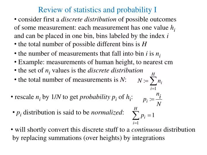
1. Review of statistics and probability I • consider first a discrete distribution of possible outcomes of some measurement: each measurement has one value hi and can be placed in one bin, bins labeled by the index i • the total number of possible different bins is H • the number of measurements that fall into bin i is ni • Example: measurements of human height, to nearest cm • the set of ni values is the discrete distribution • the total number of measurements is N: • rescale ni by 1/N to get probabilitypi of hi: • pi distribution is said to be normalized: • will shortly convert this discrete stuff to a continuous distribution • by replacing summations (over heights) by integrations

2. Review of statistics and probability II • if we lined up all the people end to end we would obtain the total length L: • what is the average deviation? What does it tell us? • the average height of a person is <h>: • and this is a paradigm for calculating ANY average! • How narrow or broad is the distribution? • the deviationi of a measurement hifrom the average := hi– <h> • it tells us NOTHING about the “spread” of the distribution

3. Review of statistics and probability III • consider the squared deviationi:= (hi- <h>)2 • this is always ≥ 0 • now consider the average of this quantity: the variance • the square root of this quantity is the standard deviation, with the same units as the quantity in question • it will turn out to be the uncertainty in a measurable

4. Now convert to a continuous distribution • now the bin index is a continuous variable: i  x • now the sums from i =1 to i = H become integrals over the domain of x (say, –∞ ≤ x ≤ ∞) • define the probability density r(x) as follows: the probability that a measurement of x occurs between x and x + dx is r(x) dx • the dimensions of r(x) are the dimensions of 1/x • r(x) distribution is said to be normalized: • probability that measurement x is between a and b: • average value of x in that interval a < x < b: • average value of f(x) in that interval a < x < b:

5. Application of these ideas to the black body radiator • we assume that a cavity with a small hole acts as a perfect black body, since any radiation (light) that strikes the hole is ‘absorbed’… so whatever light comes out of the hole is characteristic of black body radiation • if one ‘counts standing wave modes’ in a cavity of volume V, it may be shown that the number of modes in frequency range df is expressed as a probability-like distribution • for a system to possess an energy E when in an environment at temperature T, the probability that its energy is within dE is expressed by the Boltzmann factor: • When this is normalized, it is easy to show A = 1/kT • average energy is therefore

6. The wrong black body theory and its repair • Now we make an incorrect but reasonable assumption: assume that each mode can have any energy E at all, as long as the average in the mode is that average energy kT (thus, consistent with the Boltzmann probability), so that the amount of energy in frequency range df is h(f) kT df: • this ‘energy-per-frequency’ function e(f), unfortunately, diverges to infinity as f ∞, and so does its integral over all frequencies, which would be the total energy in the cavity! • both problems are collectively termed the ultraviolet catastrophe! • to fix the problem, Planck proposed that the mode energy E is restricted to only be an integer times a constant times the frequency: E = nhf, and the value of h will be determined by the data • thus, the mode energy is quantized so now are statistics are those of a discrete distribution: we say that each mode contains an integer # of photons appropriate to its frequency

7. Implications of quantizing a mode’s energy • again we invoke Boltzmann, and say that the probability for a mode to have energy E is • of course, we must normalize this discrete probability distribution: • so the probability to have energy E is • now we can find the average energy of a mode as usual:

8. The UV catastrophe has vanished! • assembling all the pieces we arrive at the Planck distribution • drops to zero for large f like • drops to zero for small f like f3