Download
1 / 20
200 likes | 351 Views
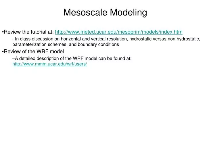
Mesoscale Modeling. Review the tutorial at: http://www.meted.ucar.edu/mesoprim/models/index.htm In class discussion on horizontal and vertical resolution, hydrostatic versus non hydrostatic, parameterization schemes, and boundary conditions Review of the WRF model

E N D
Mesoscale Modeling Review the tutorial at: http://www.meted.ucar.edu/mesoprim/models/index.htm In class discussion on horizontal and vertical resolution, hydrostatic versus non hydrostatic, parameterization schemes, and boundary conditions Review of the WRF model A detailed description of the WRF model can be found at: http://www.mmm.ucar.edu/wrf/users/
WRF Model Overview - What are the important physical processes that are resolved in the WRF model? In the atmosphere, the equations of motion are solved for u,v,w Turbulence and turbulent mixing A thermodynamic equation to predict potential temperature Long and short wave radiation Clouds – either explicitly resolved (qv,qc,qr,qi,qs,qg) or parameterized if the horizontal grid spacing is greater than about 10 km A boundary layer scheme that handles the generation of boundary layers eddies that transport heat, moisture, and momentum through the boundary layer. A surface layer scheme handles the fluxes of heat, and moisture from the surface to the atmosphere. It also interacts with the radiation scheme as long/short wave radiation is emitted, absorbed, or scattered from the earth’s surface A land surface scheme that may contain a soil moisture model. It may also resolve the type of vegetation on the surface, ice, sea ice, and snow Other Features: Data Assimilation WRF-Chem model Grid nesting
WRF Model Overview - What do the model equations look like? Note that the equations below are NOT complete. For example, they do not contain any moisture variables.
WRF Model Overview - The complete model equations are then written in finite difference form to be solved numerically. What does the model grid look like? (figures from the WRF-ARWV2 Users Guide)
WRF Model Overview - The Vertical Coordinate: The eta surfaces are often packed close together where higher vertical resolution is required – such as near the surface and up at tropopause level. (figures from the WRF-ARWV2 Users Guide)
WRF Model Overview - Nam DOMAIN WRF DOMAIN To run the model, it needs to be initialized with the current atmospheric state. How is this done? Often with the analysis generated by a coarser, larger scale NWP model such as the Nam or GFS: You can run WRF as a global model.
WRF Model Overview - Nam DOMAIN Information such as u,v,w passed from Nam to WRF model lateral boundary periodically during model run WRF DOMAIN As the WRF model runs, it will periodically (often every 3 hours) need information from the coarse model (Nam) at the lateral boundaries to account for information passing into and out of the WRF model domain:
WRF Model Overview - (figures from the WRF-ARWV2 Users Guide) Within WRF, and many other mesoscale models, you can nest a finer-scale grids within the outer domain:
WRF Model Overview - This is what the model grids would look like: (figures from the WRF-ARWV2 Users Guide)
WRF Model Overview - Physics options available within WRF Microphysics Cumulus parameterizations Surface layer physics Land surface model Boundary layer Long and short wave radiation Let’s examine these in more detail:
WRF Model Overview - Microphysical Processes – how does the model handle clouds and precipitation?
WRF Model Overview - Microphysical Processes – how does the model handle clouds and precipitation? In WRF, you have 7 different options: They all parameterize microphysical processes differently. The variables represented are not all the same for the different schemes. Let’s run WRF using the Kessler warm rain scheme and the Lin ice scheme for a supercell simulation The prognostic variables for these schemes include qv,qc,qr,qi,qs,qg Single moment Mixing ratios and number distributions (table from the WRF-ARWV3 Users Guide)
WRF Model Overview - If the grid spacing is greater than say 5-10 km, the model resolution is to coarse to resolve convective cells explicitly. In this situation, clouds and precipitation are produced by cumulus parameterization schemes. Parameterization: The representation, in a dynamical model, of physical effects in terms of admittedly oversimplified parameters, rather than realistically requiring such effect to be consequences of the dynamics of the system. (from Glossary of Meteorology online) In WRF, you have four cumulus parameterization processes to choose from
WRF Model Overview - The surface layer: The surface layer scheme handles the fluxes of heat, moisture and momentum from the model surface to the boundary layer above. There are three surface layer options available within WRF
The land-surface models (LSMs) use atmospheric information from the surface layer scheme, radiative forcing from the radiation scheme, and precipitation forcing from the microphysics and convective schemes, together with internal information on the land’s state variables and land-surface properties, to provide heat and moisture fluxes over land points and sea-ice points. These fluxes provide a lower boundary condition for the vertical transport done in the PBL schemes (or the vertical diffusion scheme in the case where a PBL scheme is not run, such as in large-eddy mode). [Note that large-eddy mode with interactive surface fluxes is not yet available in the ARW, but is planned for the near future.] The land-surface models have various degrees of sophistication in dealing with thermal and moisture fluxes in multiple layers of the soil and also may handle vegetation, root, and canopy effects and surface snow-cover prediction. The landsurface model provides no tendencies, but does update the land’s state variables which include the ground (skin) temperature, soil temperature profile, soil moisture profile, snow cover, and possibly canopy properties. There is no horizontal interaction between neighboring points in the LSM, so it can be regarded as a one-dimensional column model for each WRF land grid-point, and many LSMs can be run in a stand-alone mode.(text from the WRF-ARWV3 Users Guide) WRF Model Overview - The Land Surface Model (LSM):
Figure from RAP/NCAR WRF Model Overview - • WRF has the option to couple an urban canopy model to this LSM • Street canyons – urban geometry • Shadowing from building and radiation reflection • Urban winds in canopy layer • Heat equation for roof wall and road surfaces. One of the land surface models available in WRF:
WRF Model Overview - There are three land surface models available in WRF: (table from the WRF-ARWV3 Users Guide) Can couple an ocean mixed-layer model to this scheme (for hurricane modeling)
WRF Model Overview - Boundary Layer Schemes: In the real atmosphere, turbulent eddies transport heat, moisture, and momentum through the boundary layer: Unless the horizontal grid spacing is a few hundred meters or less, these eddies are two small to be resolved in the model Therefore, the boundary layer scheme tries to parameterize these eddies and their role in transporting heat, moisture, and momentum. There are four boundary layer schemes available within WRF
The radiation schemes provide atmospheric heating due to radiative flux divergence and surface downward longwave and shortwave radiation for the ground heat budget. Longwave radiation includes infrared or thermal radiation absorbed and emitted by gases and surfaces. Upward longwaveradiative flux from the ground is determined by the surface emissivity that in turn depends upon land-use type, as well as the ground (skin) temperature. Shortwave radiation includes visible and surrounding wavelengths that make up the solar spectrum. Hence, the only source is the Sun, but processes include absorption, reflection, and scattering in the atmosphere and at surfaces. For shortwave radiation, the upward flux is the reflection due to surface albedo. Within the atmosphere the radiation responds to model-predicted cloud and water vapor distributions, as well as specified carbon dioxide, ozone, and (optionally) trace gas concentrations. All the radiation schemes in WRF currently are column (one-dimensional) schemes, so each column is treated independently, and the fluxes correspond to those in infinite horizontally uniform planes, which is a good approximation if the vertical thickness of the model layers is much less than the horizontal grid length. This assumption would become less accurate at high horizontal resolution. WRF Model Overview - Long and Short-wave Radiation
WRF Model Overview - Long and Short-wave Radiation There are currently 7 radiation schemes available in WRF