Download
1 / 27
270 likes | 383 Views
Presentation at P. P. Shirshov Institute of Oceanology, Moscow, Russia November 11, 2011. Climatic Effects of Mesoscale Turbulence in the Ocean and Atmosphere. Sergey Kravtsov

E N D
Presentation at P. P. Shirshov Institute of Oceanology, Moscow, Russia November 11, 2011 Climatic Effects of Mesoscale Turbulence in the Ocean and Atmosphere Sergey Kravtsov University of Wisconsin-Milwaukee Department of Mathematical Sciences Atmospheric Science Group Collaborators: I. Kamenkovich, University of Miami, USA; A. Hogg, Australian National University, Australia; M. Wyatt, University of Colorado, USA, A. A. Tsonis, K. Swanson, C. Spannagle, N. Schwartz, J. M. Peters, University of Wisconsin-Milwaukee, USA http://www.uwm.edu/kravtsov/
My background and research interests 1993 — MIPT, MS: Singular barotropic vortex on a beta-plane (G. M. Reznik, MS advisor) 1998 — FSU, PhD: Coupled 2-D THC/sea-ice models (W. K. Dewar, PhD advisor) • 1998–2005 — UCLA, PostDoc: Atmospheric regimes, wave–mean-flow interaction, coupled ocean–atmosphere modes (M. Ghil, post-doc advisor; A. Robertson, J. C. McWilliams, P. Berloff, D. Kondrashov)
2005–present — University of Wisconsin-Milwaukee (UWM), Dept. of Math. Sci., Atmospheric Science group: Multi-scale climate variability: atmospheric synoptic eddies/LFV (S. Feldstein, S. Lee, N. Schwartz, J. Peters), oceanic mesoscale turbulence/large-scale response (W. Dewar, A. Hogg, P. Berloff, I. Kamenkovich, J. Peters) Model reduction (D. Kondrashov, M. Ghil, A. Monahan, J. Culina) Regional climates and global teleconnections (C. Spannagle, A. Tsonis, K. Swanson, M. Wyatt, P. Roebber, J. Hanrahan) Weather/climate predictability, decadal prediction
Topics to be considered Atlantic Multidecadal Oscillation and Northern Hemisphere’s climate variability (with M. Wyatt and A. A. Tsonis)* Empirical model of decadal ENSO variability* *To be presented at IFA, November 17, 2011 This talk: Predictability associated with nonlinear regimes in an idealized atmospheric model (with N. Schwartz and J. Peters) On the mechanisms of the late 20th century SST trends over the Antarctic Circumpolar Current (with I. Kamenkovich, A. Hogg, and J. Peters)
PREDICTABILITY ASSOCIATED WITH NONLINEAR REGIMES IN AN IDEALIZED ATMOSPHERIC MODEL J. Peters, S. Kravtsov, and N. Schwartz (Journal of the Atmospheric Science, accepted October 2, 2011)
Atmospheric flow regimes x — large-scale, low-frequency flow x’ — fast transients, F — external forcing N3 can be approximated as Gaussian noise If N1 and N2are small or linearly parametrizable, x will also be Gaussian-distributed Deviations from gaussianity — REGIMES — can be due to N1, N2 and F
Two paradigms of regimes Regimes are due to deterministic non-linearities(e.g., Legras and Ghil ‘85) Regimes are due to multiplicative noise (Sura et al. ’05) The first type of regimes is inheren-tly more predictable
Is there enhanced predictability associated with regimes? We address this ques-tion by studying the out-put from a long simula-tion of a three-level QG model(Marshall&Molteni ’93) The QG3 model is tuned to observed clima-tology and has a realistic LFV with non-gaussian regimes(Kondrashov et al.)
Regime Identification Regimes defined as regions of enhanced probability of persistence relative to a benchmark linear model (cf. Vautard et al. ’88; Kravtsov et al. ‘09), in Uz200 and Psi200 EOF-1–EOF-2 subspaces
Four Distinct Regimes in QG3 model AO Regimes 1 and 2 are largely zonally symmetric and stati-stically the same bwn the two metrics 1: AO+ 2: AO– Non-AO Regimes 3 in Uz and Psi are less zonally sym-metric; they are distinct regimes Uz 3: N-AO+ Psi 3: NAO+ Similar regimes were obtained before
Regimes and Predictability “Predictable” R1 and R2 have precursor regions of low RMSD (blue areas in fig.) 3 2 1 Same precursor regions for lead 5 and 10-day fcst Initializations in precursor regions end up in regimes
Regime 1 Regime 2 Predictable regimes: Day 1 Initializations from precursor regions slow down in regime regions and stay there, while maintaining low spread Day 5 Day 10
Non-regime Regime 3 Unpredictable states: Day 1 Initializations from non-precursor regions spread out faster and quickly decay to climatology Day 5 Day 10
Discussion Regimes are not always associated with enhanced predictability (cf. Sura et al. ‘05) In QG3, the predictable regimes arise as a combination of (i) nonlinear slowdown of trajectories’ decay toward climatology (deterministic nonlinearity) and(ii) reduced spread of trajectories in regime regions (multiplicative noise). Unpredictable regimes don’t have (ii). Detailed effects of deterministic nonlinearity and multiplicative noise onto predictability are studied by fitting a nonlinear stochastic SDE to the QG3 generated time series (Peters and Kravtsov 2011)
ON THE MECHANISMS OF THE LATE 20TH CENTURY SST TRENDS OVER THE ANTARCTIC CIRCUMPOLAR CURRENT S. Kravtsov, I. Kamenkovich, A. Hogg, J. Peters (J. Geophys. Res. Oceans, in press)
Response of the Antarctic Circumpolat Current (ACC) to intensifying jet stream • Hogg et al. (2008) demonstrated in an idealized, but eddy- resolving three-layer model that linearly increasing wind stress causes no change in the ACC transport!
Response of ACC to increasing wind-stress II: “eddy saturation” ACC transport does not change Instead, eddy field intensifies • Enhanced eddy mixing modifies both surface and subsurface climate-change signatures, e.g., temperature trends • These conjectures based on the idealized model simulations were confirmed using more complete eddy-resolving models and observations
Estimates of the eddy effects on SST in Hogg et al. (2008) model • Typical eddy-driven SST trends forced by wind-stress trends similar to the observed (10% per decade) are 0.1–0.2 ºC per decade
SST trends over ACC: Observations and simulations by coarse-resolution global climate models SST trends match, but wind-stress trends don’t! (despite!)
Hypothesis to explain discrepancies: • Global climate models make two compensating errors to achieve seemingly correct SST trends over the ACC: • The wind-stress trends are much underestimated due, presumably, to incompleteness of anthropogenic forcing in many of the models comprising the present ensemble • The models misrepresent eddies and cannot capture trends in eddy-induced lateral mixing
“Eddies” in coarse-resolution models: GM parameterization • u* and w* — eddy-induced transports z-coordinates: Isopycnal coordinates:
Application of GM scheme in global climate models • Resulted in solutions without climate drift, in part due to improvements in the ACC region • The GM scheme needs to be turned off in the mixed layer, where the slopes of isopycnals are steep. Slope-limiting and/or taper functions were typically used • Non-constant K(x, y, z, t) have been suggested. We argue that this is essential to model ACC changes forced by wind-stress trends in coarse- resolution models
SST response in a coarse-res. ocean model No change in wind • The “eddy-induced” response magnitude consistent with that in idealized eddy- resolving model Observed wind changes • The SST trends due to various forcings combine linearly • Linearly increasing K and KH (in mixed layer)
Conclusions • The ACC operates in an eddy-saturated regime: increasing wind-stress forcing does not accelerate the time-mean current, but energizes eddy field • The enhanced eddy mixing induces quantitatively important SST trends in the region • This effect can be parameterized in coarse-grid climate models via variable GM and lateral diffusion coefficients. Such schemes are not implemented in many of these models... (or maybe it’s better to just resolve eddies!) Correct simulation of surface response in the ACC region to various forcings has numerous implications for accurate climate prediction (coupled modes, CO2 sinks etc.)