Download
1 / 43
430 likes | 575 Views
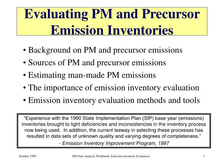
Evaluating PM and Precursor Emission Inventories. Background on PM and precursor emissions Sources of PM and precursor emissions Estimating man-made PM emissions The importance of emission inventory evaluation Emission inventory evaluation methods and tools.

E N D
Evaluating PM and Precursor Emission Inventories • Background on PM and precursor emissions • Sources of PM and precursor emissions • Estimating man-made PM emissions • The importance of emission inventory evaluation • Emission inventory evaluation methods and tools “Experience with the 1990 State Implementation Plan (SIP) base year (emissions) inventories brought to light deficiencies and inconsistencies in the inventory process now being used. In addition, the current leeway in selecting these processes has resulted in data sets of unknown quality and varying degrees of completeness.” - Emission Inventory Improvement Program, 1997 PM Data Analysis Workbook: Emission Inventory Evaluation
What is Particulate Matter and How Does it Vary? Husar, 1999 • What is Particulate Matter? • How Does PM Vary? PM Data Analysis Workbook: Emission Inventory Evaluation
What is Particulate Matter? What is particulate matter and where does it come from? The term Particulate Matter or aerosol, refers to liquid or solid particles suspended in the air. Depending on their origin and visual appearance, aerosols have acquired different names in the everyday language. Dust refers to solid airborne material, dispersed into aerosol from grainy powders such as soil. Combustion processes produce smoke particles, but the incombustible residues of coal are called flyash. Particles of size 2.5 um and smaller are referred to as PM2.5. PM2.5 is composed of a mixture of primary and secondary compounds. Primary particulate PM2.5 compounds consist of soil-related, inorganic, elemental, and organic carbonaceous particles emitted directly into the atmosphere by fossil fuel combustion, biomass combustion, and mechanical processes. Secondary particulate compounds are formed in the atmosphere via chemical reactions of particulate precursors (VOC, SO2, NOx, SOA, and NH3) emitted by many combustion and non-combustion sources. The principal types of secondary particles are ammonium sulfate and ammonium nitrate formed in the atmosphere from gaseous emissions of SO2 and NOx reacting with NH3. In the early days, air pollution had the appearance of both smoke and fog, so the term smog was created. In the open atmosphere, the visibility may often be reduced by regional haze, originating from various natural or anthropogenic sources. Neither water droplets of fog and clouds, snow, rain, sleet (hydrometors) nor dust particles larger than 100 um (blowing sand) are considered to be particulate matter. How does PM vary spatially, temporally, with particle size, and by chemical composition? As all pollutants, the ambient aerosol concentration patterns contain endless variability in space and time. However, unlike gaseous pollutants, particulate matter also depends on particle size, shape and chemical composition. The chemically rich aerosol mix arises from the multiplicity of PM sources, each having a unique chemical signature at the source. These chemical signatures are referred to as chemical speciation profiles. The primary aerosol chemical composition is further enriched by the addition of secondary species during atmospheric transport. The effective mixing in the lower atmosphere stirs these primary and secondary particles into an externally mixed batch with various degrees of homogeneity, depending on location and time. Lastly, repeated cloud scavenging and evaporation tends to mix the particles from different sources internally into particles with mixed composition. The result is a heterogeneous PM mixture that is probably unparalleled in the domain of atmospheric sciences. For instance it is common to find soot particles within sulfate droplets, or nitrate deposited on sea salt particles. Husar, 1999 PM Data Analysis Workbook: Emission Inventory Evaluation
PM2.5 Background and Terminology (1 of 3) • The term Particulate Matter (PM) or aerosol, refers to liquid or solid particles suspended in the air; PM2.5 refers to particles of size 2.5 m and smaller. • Dust refers to solid airborne material, dispersed into aerosol from grainy powders such as soil. • Combustion processes produce smoke particles, but the incombustible residues of coal are called flyash. • In the open atmosphere, the visibility may often be reduced by regional haze, originating from various natural or anthropogenic sources. Husar, 1999 PM Data Analysis Workbook: Emission Inventory Evaluation
PM2.5 Background and Terminology (2 of 3) • PM2.5 is composed of a mixture of primary and secondary compounds. • Primary particulate PM2.5 consists of soil-related, inorganic, elemental, and organic carbonaceous particles emitted directly into the atmosphere by fossil fuel and biomass combustion, and mechanical processes. • Secondary particulate compounds are formed in the atmosphere via chemical reactions of particulate precursors (VOC, SO2, NOx, SOA, and NH3) emitted by many combustion and non-combustion sources. PM Data Analysis Workbook: Emission Inventory Evaluation
PM2.5 Background and Terminology (3 of 3) • The principal types of secondary particles are ammonium sulfate and ammonium nitrate formed in the atmosphere from gaseous emissions of SO2 and NOx reacting with NH3. • There is a direct relationship between the particle size and the atmospheric residence time of particles: PM Data Analysis Workbook: Emission Inventory Evaluation
Urban Sources of PM2.5 and Precursor Emissions • Motor vehicle exhaust • Paved road dust • Fossil fuel fired boilers at electric utility plants • Residential wood combustion • Entrained geologic material PM Data Analysis Workbook: Emission Inventory Evaluation
Characteristics of PM (1 of 2) • Many sources of PM are seasonal (e.g., residential wood combustion, dust sources, forest fires). • Meteorology impacts the formation of secondary PM. • The formation of secondary PM involving OH, O3, and H2O2, species which are normally present in the atmosphere but which are present in higher concentrations during periods of increased sunlight and temperature, peaks during the summer in most U.S. areas. • The formation of secondary PM can be affected by the water content of the atmosphere; higher water content facilitates the formation of certain secondary particles, consequently, PM also tends to be a problem in the winter. EPA, 1996 PM Data Analysis Workbook: Emission Inventory Evaluation
Characteristics of PM (2 of 2) • Primary and secondary PM2.5 have long lifetimes in the atmosphere (days to weeks) and travel long distances (hundreds to thousands of kilometers). • PM2.5 particles tend to be uniformly distributed over urban areas, as a result, they are not easily traced back to their individual sources. • Natural sources of background PM include: wind blown dust from erosion and re-entrainment; long range transport of dust from the Sahara desert; sea salt; particles formed from the oxidation of sulfur compounds emitted from oceans and wetlands; the oxidation of NOx from forest fires; and the oxidation of VOC compounds emitted by plants and trees. EPA, 1996 PM Data Analysis Workbook: Emission Inventory Evaluation
PM and Precursor Emission Inventories Purpose of PM emission inventory development: • Used by regulatory community • Air quality modeling support (model input) • Exposure modeling support, health assessment • Control cost analysis • Regulatory control strategy development “The Clean Air Act requires state and local air quality agencies to develop complete and accurate inventories as an integral part of their air quality management responsibilities. These air emission inventories are used to evaluate air quality, track emissions reduction levels, and set policy on a national and regional scale...” - Emission Inventory Improvement Program, 1997 PM Data Analysis Workbook: Emission Inventory Evaluation
Emission Inventory Development (1 of 4) • Estimating PM2.5 emissions is a complex process involving many data parameters. • Uncertainties in emissions inventory estimates could range from about 10% for well defined sources (e.g., emissions from power plants) to an order of magnitude for widespread and sporadic sources (e.g., fugitive dust). • General equation for estimating emissions gets complex when estimating PM: E = A x EF x (1-ER/100) Where: E = emissions EF = emission factor A = activity ER = overall emission reduction efficiency (%) PM Data Analysis Workbook: Emission Inventory Evaluation
Emission Inventory Development (2 of 4) Spatial Allocation of Emissions Activities • Emissions sources are spatially allocated to a region using the actual locations of the emissions sources, and/or using spatial surrogate data which are physical parameters that can be associated with emissions activities (e.g., acres of farmland might be the surrogate for emissions from farming operations) Temporal Allocation of Emissions Activities • Emissions sources are temporally allocated by assigning a temporal profile, a distribution of emissions activity over a 24-hour period, to each source category. PM Data Analysis Workbook: Emission Inventory Evaluation
Emission Inventory Development (3 of 4) Chemical Speciation of Emissions Sources • In order to disaggregate PM emissions into individual chemical species, each emissions source category is assigned a speciation profile which provides a detailed chemical breakdown of the individual chemical species emitted from that source. • Several sources of PM speciation data currently exist including: • EPA’s SPECIATE: (http://www.epa.gov/ttn/chief/software.html#speciate) • U.C. Davis (via California ARB): (http://www.arb.ca.gov/emisinv/speciate/pmucd.pdf) • DRI: (http://www.dri.edu) • OMNI (via California ARB): http://www.arb.ca.gov/emisinv/speciate/pmomni.pdf PM Data Analysis Workbook: Emission Inventory Evaluation
Emission Inventory Development (4 of 4) Challenges in developing PM2.5 emission inventories • Limited PM2.5 activity and emission factor data • Variable quality of existing PM2.5 data • Estimation of secondary PM2.5 PM Data Analysis Workbook: Emission Inventory Evaluation
The Importance of Evaluating Emissions Estimates • Reviewing and evaluating emissions inventories is critical because development of effective air pollution control strategies is predicated on the accuracy of the underlying emission inventory. • Uncertainties associated with PM2.5 emissions estimates can range from 10% to an order of magnitude. • Emissions data commonly contain errors in pollutant mass. • Quality control and assurance of emissions estimates can significantly improve the quality of the data. PM Data Analysis Workbook: Emission Inventory Evaluation
The Importance of Emission Inventory Evaluation Why bother evaluating emissions data? Emission inventory development is a complex process that involves estimating and compiling emissions activity data from hundreds of point, are, and mobile sources in a given region. Because of the complexities involved in developing emission inventories, and the implications of errors in the inventory on air quality model performance and control strategy assessment, it is important to evaluate the accuracy and representativeness of any inventory that is intended for use in air quality modeling. Furthermore, existing emission factor and activity data for sources of PM2.5 are limited and the quality of the data is questionable. An emission inventory evaluation should be performed before the data are used in photochemical modeling. What tools are available for assessing emissions data? There are several techniques used to evaluate emissions data including: “common sense” review of the data, source-receptor methods such as CMB8, bottom-up evaluations that begin with emissions activity data and estimate the corresponding emissions, and top-down evaluations that compare emissions estimates to ambient air quality data. Each evaluation method exhibits strengths and limitations. Based on the results of the emissions evaluation, recommendations can be made on possible improvements to the emission inventory. Local agencies responsible for developing the inventory can then make revisions to the inventory data prior to air quality modeling. PM Data Analysis Workbook: Emission Inventory Evaluation
Use of mathematical techniques to evaluate emissions estimates: Engineering judgement approach Bottom-up emissions evaluation Use of ambient air quality data to evaluate and reconcile emissions estimates: Multivariate Techniques - Principal Component Analysis (PCA) receptor modeling, Chemical Mass Balance (CMB) receptor modeling Top-down emissions evaluation Emission Inventory Evaluation Tools and Methods PM Data Analysis Workbook: Emission Inventory Evaluation
Strengths Limitations Using Engineering Judgement to Evaluate Emissions Estimates (1 of 2) • Begin with knowledge of the region for which the emission inventory was developed (i.e., likely emissions sources, population, demographic characteristics). • Review major sources of emissions and perform per-capita checks combined with conventional wisdom to evaluate emissions data. • Provides a quick and inexpensive method to quality control emissions estimates • Does not require extensive data • Can quickly identify gross errors in emissions data • Can identify errors in emissions data, gives no insight as to where errors emanate PM Data Analysis Workbook: Emission Inventory Evaluation
Summer emission inventories often report significant emissions from seasonal sources such as residential fireplaces and wood stoves and snowmobiles. Residential fireplace and wood stove emissions in the summer? Case Study: Using Engineering Judgement to Evaluate Emissions Estimates (2 of 2) Residential fireplaces and wood stoves are large contributors to PM emissions in the wintertime. Emissions contributions from this source should be low in the summer months. Taking the time to review seasonal emission inventory data can catch errors like this. PM Data Analysis Workbook: Emission Inventory Evaluation
Strengths Limitations Bottom-up Emission Inventory Evaluation (1 of 2) • Method of assessing emissions data using census information and emissions activity data combined with emission factors to generate independent estimates to compare to existing data. • This method is most useful when combined with the top-down evaluation when assessing large data sets. Top-down identifies problem categories, bottom-up used to investigate underlying information used to estimate categories. • The emission estimates generated using this methodology can be very accurate if demographic and activity data are accurate. • Extensive data requirements. • Accuracy of emission factors • Accuracy of activity data • Time consuming. PM Data Analysis Workbook: Emission Inventory Evaluation
Mobile source emissions activity data for anonymous city: Urban region with a total fleet of 366,699 on-highway motor vehicles. Emissions data reported that 494 of these vehicles are heavy-duty diesel trucks (HDDTs). According to these figures, 0.1% of the vehicle fleet are HDDTs. Case Study: Bottom-up Evaluation of Emissions Activity Data (2 of 2) Bottom-up Emission Inventory Evaluation (2 of 2) In other parts of the country with similar characteristics, HDDTs make up approximately 10 to 20 percent of highway vehicles. HDDTs are significant contributors to PM, consequently, errors in activity data can lead to errors in emissions estimates. Adapted from Haste et. al., 1998 PM Data Analysis Workbook: Emission Inventory Evaluation
Issues Associated With Emissions EvaluationsUsing Ambient Data Ambient air quality data can be used to evaluate emissions estimates and source apportionment, however, the following issues should be considered: • Proper spatial and temporal matching of emissions estimates and ambient data. • Ambient levels of background PM2.5. • Meteorological effects on comparison. • Comparisons only valid for primary PM2.5. • Temporal resolution of ambient data (i.e., 24-hour average versus hourly ambient PM data) PM Data Analysis Workbook: Emission Inventory Evaluation
Strengths Limitations Multivariate Analyses (1 of 2) • Statistical procedures that can be used to infer mix of PM sources impacting a receptor location. • Procedures including cluster, factor/principal component, regression, and other multivariate techniques available in statistical software packages. • Simple statistical methods. • Does not require speciation profile data. • Ability to summarize multivariate data set using few components. • Identifies unusual ambient samples. • Does not apportion secondary aerosol. • Analyst must infer how certain statistical species groupings relate to emissions sources • Depends on correlation that can be driven by meteorology or co-location. API, 1998 PM Data Analysis Workbook: Emission Inventory Evaluation
Multivariate Analysis Sample Output (2 of 2) Example analysis to be added PM Data Analysis Workbook: Emission Inventory Evaluation
Overview of Receptor Models Receptor Models: provide empirical relationships between ambient data at a receptor and PM emissions by source category. The fundamental principal of receptor modeling is that mass conversion is assumed and a mass balance analysis is used to identify and apportion sources of PM in the atmosphere. Receptor models are useful for resolving composition of ambient primary PM into components related to emissions sources. Three main types of receptor models: • Models that apportion primary PM using source information • Models that apportion primary PM without using source information • Models that apportion primary and secondary PM There are more than a dozen currently existing receptor models, however, EPA’s OAQPS has only recognized CMB and PCA as part of their SIP development guidance documents. API, 1998 PM Data Analysis Workbook: Emission Inventory Evaluation
The Chemical Mass Balance Receptor Model (1 of 4) • The CMB uses the chemical and physical characteristics of gasses and particles measured at sources and receptors to both identify the presence of and to quantify source contributions to receptor concentrations. • CMB calculations are based on fact that many chemical species in the atmosphere do not participate in rapid chemical reactions in the atmosphere, so they have the same chemical form as when they were emitted. • These chemical species can be used in a three-step procedure to apportion the ambient pollutants to the sources from which they were emitted. Watson et. al., 1998 PM Data Analysis Workbook: Emission Inventory Evaluation
The Chemical Mass Balance Receptor Model (2 of 4) Three step source apportionment using CMB: Step 1: Measure chemical composition of emissions for the important sources of PM2.5 (e.g., diesel engines, suspended road dust, coal-fired boilers). These chemical composition data are called source profiles. There are several existing libraries of source profile data. Step 2: Collect and analyze samples of chemical species in the ambient air. Step 3: Apply the CMB model to each ambient sample to determine the relative amounts of emissions from each type of source, which, when mixed together give the best agreement with the measured composition of the atmosphere. Each item of input data is accompanied by an estimate of its uncertainty. The CMB model combines these uncertainties to calculate the uncertainty in each output value that is attributable to the uncertainties in the input data. Watson et. al., 1998 PM Data Analysis Workbook: Emission Inventory Evaluation
Strengths The Chemical Mass Balance Receptor Model (3 of 4) Limitations • User friendly model. • CMB8 (version 8) operates in a Windows-based environment and accepts inputs and creates outputs in a wide variety of formats. • Accepted by EPA’s OAQPS for SIP development. • Generates errors in source compositions accepted by OAQPS • Requires source profile information. • Results of CMB model are only as accurate as the speciation profile input data. • Significant portion of PM2.5 mass is due to secondary compounds which are not apportioned by CMB. • Can mis-specify emissions sources. • Sensitive to collinearity. PM Data Analysis Workbook: Emission Inventory Evaluation
Comparison of CMB modeling results and emission inventory source apportionment are very different. The results of CMB modeling show that mobile sources are responsible for a much larger percentage of PM2.5 in the ambient air while the emission inventory data shows dust being the main contributor to PM2.5. These types of discrepancies are important to consider prior to control strategy development. Case Study: Using CMB to Assess Emissions Estimates and Source Apportionment (4 of 4) Emission Inventory PM2.5 Source Apportionment CMB PM2.5 Source Apportionment Lurmann et. al., 1999 Watson et. al., 1998 PM Data Analysis Workbook: Emission Inventory Evaluation
Top-Down Emission Inventory Evaluation (1 of 6) Top-Down Emissions Evaluation: method of comparing emissions estimates with ambient air quality data. Ambient/emission inventory comparisons are useful for examining the relative composition of emission inventories; they are not useful for verifying absolute pollutant masses unless they are combined with bottom-up evaluations. The top-down method has demonstrated success at reconciling emissions estimates of VOC and NOx, however, using the top-down method for PM is currently being explored. Top-Down Approach for PM: • Compare morning (e.g., 7:00-9:00 am) ambient- and emissions-derived primary PM2.5 /NOx ratios. Early morning sampling periods are the most appropriate to use in these evaluations because emissions are generally high, mixing depths are low, winds are usually light, and photochemical reactions are minimized. PM Data Analysis Workbook: Emission Inventory Evaluation
Ambient Data Requirements Select ambient monitoring sites dominated by fresh urban source emissions. Validate and process elemental PM data. Select early morning (e.g., 7:00-9:00 am) hourly data. Analyze meteorological data to determine the emission areas and elevated point sources that may influence ambient measurements. Top-Down Emission Inventory Evaluation (2 of 6) Emissions Data Requirements • Evaluate emissions for same locations as ambient monitor. • Process emissions data to get gridded, hourly PM2.5 data. • Convert emissions data units to be compatible with ambient data units. • Existing emissions processing software: EPS 2.0, SMOKES, EMS-95 PM Data Analysis Workbook: Emission Inventory Evaluation
Top-Down Emission Inventory Evaluation (3 of 6) Analyses: • Compare ambient data with emission estimates from different wind quadrants surrounding the monitoring site. • Compare ambient data with emission estimates with and without elevated point-source emissions. The inclusion of elevated point sources will depend on the meteorological conditions. • Perform primary PM2.5/NOx ratios for day specific, weekday, and weekend data. • Compare individual chemical species in the ambient air to chemical species in the emission inventory when speciation data is available. PM Data Analysis Workbook: Emission Inventory Evaluation
Top-Down Emission Inventory Evaluation (4 of 6) Wind Quadrant Definitions Used in the Top-down Evaluation PM Data Analysis Workbook: Emission Inventory Evaluation
Top-Down Emission Inventory Evaluation (5 of 6) • Estimating primary PM2.5 in the ambient air using chemistry data: • [Primary PM2.5] = 1.89*[Al] + 1.57*[Si] + 1.2*[K] + 1.4*[Ca] + 1.43*[Fe] + EC + 0.7*(1.4*OC) • Where: • [Al] = concentration of aluminum [Si] = concentration of silica • [K] = concentration of potassium [Ca] = concentration of calcium • [Fe] = concentration of iron EC = elemental carbon • OC = organic carbon • The multipliers in the equation account for the extra mass of oxygen in the crustal oxides and for the extra mass of hydrogen and oxygen with the organics. • It is estimated that 70 to 90 percent of organic carbon is primary. Kumar and Lurmann, 1996 PM Data Analysis Workbook: Emission Inventory Evaluation
Top-Down Emission Inventory Evaluation (6 of 6) Uncertainty Issues: • Proper temporal and spatial matching of emissions data and ambient data. • Meteorological factors including temperature, wind speed, and inversion height. • Level of ambient background PM and precursor concentrations due to transport and carry-over. • Co-location of emissions sources. • Uncertainties associated with primary versus secondary PM. • Underlying assumption that emission inventory NOx estimates are reasonable. PM Data Analysis Workbook: Emission Inventory Evaluation
Case Study: Top-Down Emissions Evaluation (1 of 2) Analysis Objective • Evaluate the consistency of gridded, hourly emission inventory with ambient PM and NOx data. • Compare ambient data with emission estimates with and without elevated point-source emissions. The inclusion of elevated point sources will depend on the meteorological conditions. • Perform primary PM10/NOx ratios for day specific, weekday, and weekend data. • Identify areas of the emission inventory that appear to be inconsistent with the ambient air and make recommendations on possible improvements to the inventory. Haste et. al., 1998 PM Data Analysis Workbook: Emission Inventory Evaluation
Primary PM10/NOx Anonymous City #1 Anonymous City #2 Case Study: Top-Down Emissions Evaluation (2 of 2) Top-Down comparison of ambient- and emissions derived primary PM10/NOx in two anonymous cities. Ambient Ratio Emission Inventory Ratio Comparison of the ambient- and emissions derived PM10/NOx ratios in two anonymous cities are quite different. It appears as though PM10 is overestimated in the emission inventory by approximately a factor of two. Recommendation: the PM10 portion of the inventory should be investigated from the bottom-up. Note that this example corresponds to PM10; a similar comparison could be made for PM2.5 PM Data Analysis Workbook: Emission Inventory Evaluation Haste et. al., 1998
Strengths Top-down Emission Inventory Evaluation Limitations and Uncertainties • Extensive data requirements. • Uncertainties in the emission inventory carry-over to comparisons. • Uncertainties in the ambient data measurements carry-over to comparisons. • Comparison-related uncertainties • include: • Proper temporal and spatial matching of emissions data and ambient data. • Meteorological factors • Level of ambient background PM concentrations and chemical reactions • Provides a method to assess areas of an emission inventory that appear to be suspect; improvements can be made prior to photochemical modeling. • Can assess detailed chemical species composition between the inventory and ambient air if accurate PM species data is available. • Can greatly improve emissions estimates. PM Data Analysis Workbook: Emission Inventory Evaluation
Emission Inventory Data Sources Emissions data sources: • State and local air quality management agencies • EPA National Emissions Trends Inventory: http://www.epa.gov/ttn/chief/ei/ • Emission inventory improvement program guidance documents: http://www.epa.gov/ttn/chief/eiip/techrep.htm PM Data Analysis Workbook: Emission Inventory Evaluation
Ambient Data Sources Ambient data sources: • AIRS Data via public web: http://www.epa.gov/airsdata • AIRS AQS via registered users: register with EPA/NCC (703-487-4630) • PM2.5 websites via public web PM Data Analysis Workbook: Emission Inventory Evaluation
Meteorological Data Sources Meteorology data sources: • Meteorological parameters from NWS: http://www.nws.noaa.gov • Meteorological parameters from PAMS/AIRS AQS: register with EPA/NCC (703-487-4630) • Private meteorological agencies (e.g., forestry service, agricultural monitoring, industrial facilities) PM Data Analysis Workbook: Emission Inventory Evaluation
Summary PM Data Analysis Workbook: Emission Inventory Evaluation
References American Petroleum Institute (1998)/ Review of Air Quality Models for Particulate Matter, Technical Summary, Publication number 4669, March. Haste et. al., 1998 - personal communication Husar R. (1999) Draft PM2.5 topic summary available at http://capita.wustl.edu/PMFine/Workbook/PMTopics_PPT/PMDefinitions/sld001.htm Haste T.L., Chinkin L.R., Kumar N., Lurmann F.W., and Hurwitt, S.B. (1998) Use of ambient data collected during IMS95 to evaluate a regional emission inventory for the San Joaquin Valley. Final report prepared for the San Joaquin Valleywide Air Pollution Study Agency and the California Air Resources Board, Sacramento, CA by Sonoma Technology, Inc., Petaluma, CA, STI-997211-1800-FR, July. Kumar N. and Lurmann F.W. (1996) User’s guide to the speciated rollback model for particulate matter. Report prepared for San Joaquin Valleywide Air Pollution Study Agency, Sacramento, CA by Sonoma Technology, Inc., Santa Rosa, CA, STI-94250-1576-UG, September. Lurmann F.W., et. al., (1999) - personal communication Watson J.G., Fujita E.M., Chow J.C., Richards L.W., Neff W., and Dietrich D. (1998) Northern Front Range Air Quality Study. Final report prepared for Colorado State University, Cooperative Institute for Research in the Atmosphere, Fort Collins, CO by Desert Research Institute, Reno, NV. U.S. Environmental Protection Agency (1997)/ Quality Assurance Committee Emission Inventory Improvement Program Introduction: The Value of QA/QC, volume VI, chapter 1: January. U.S. Environmental Protection Agency (1996)/ Air Quality Criteria for Particulate Matter, chapter 1, Executive Summary: EPA 600/P-95/001aF, April. PM Data Analysis Workbook: Emission Inventory Evaluation