Download

1 / 36
360 likes | 501 Views
Utility. The pleasure people get from their economic activity. To identify all of the factors that affect utility would be virtually impossible Don’t forget the ceteris paribus assumption. Utility from Consuming Two Goods.

E N D
Utility • The pleasure people get from their economic activity. • To identify all of the factors that affect utility would be virtually impossible • Don’t forget the ceteris paribus assumption.
Utility from Consuming Two Goods • A person receives utility from the consumption of two goods “X” and “Y” which we show in functional notation by • The other things that appear after the semicolon are assumed to be held constant.
Measuring Utility • Because the real-world is constantly in flux, ceteris paribus is difficult to impose. • There is no unit of utility measurement. • However, it is possible to do a fairly complete job of studying choices without having to measure utility.
Assumptions about Utility • Basic Properties of Preferences • Preferences are complete : The assumption that an individual is able to state which of any two options is preferred. • Preferences are transitive: The property that if A is preferred to B, and B is preferred to C, then A must be preferred to C.
FIGURE 2.1: More of a Good Is Preferred to Less Quantity of Y per week ? Y* ? Quantity of X per week 0 X*
Indifference Curves A curve that shows all the combinations of goods or services that provide the same level of utility.
FIGURE 2.2: Indifference Curve Hamburgers per week A 6 B 4 E 3 C D F 2 U1 Soft drinks per wek 0 2 3 4 5 6
Movements Along an Indifference Curve • Why the negative slope? • Why the changing slope? • Willingness to trade.
Indifference Curves and the Marginal Rate of Substitution • Marginal Rate of Substitution (MRS): The rate at which an individual is willing to reduce consumption of one good when he or she gets one more unit of another good. • Also, the negative of the slope of an indifference curve. • The MRS between points A and B on U1 in Figure 2.2 is (approximately) 2.
Diminishing Marginal Rate of Substitution • In Figure 2.3 the person is willing to give up one hamburger to gain one more soft drink between points B and C. • Between points C and D, the consumer is only willing to give up ½ a hamburger to gain one more soft drink.
FIGURE 2.3: Balance in Consumption Is Desirable Hamburgers per week A 6 B G 4 3 C D 2 U1 Soft drinks per week 0 2 3 4 6
Diminishing Marginal Rate of Substitution • The MRS diminishes along an indifference curve moving from left to right. • This reflects the idea that consumers prefer a balance in consumption.
FIGURE 2.4: Indifference Curve Map for Hamburgers and Soft Drinks Hamburgers per week A 6 H 5 B G 4 U3 3 C U2 D 2 U1 Soft drinks per week 0 2 3 4 5 6
Application 2.2:Product Positioning in Marketing • One practical application of utility theory in marketing is the positioning of products in comparison with competitors. • Assume consumers have preferences for taste and crunchiness in breakfast cereal as represented by U1 in Figure 1.
Application 2.2:Product Positioning in Marketing • One practical application of utility theory in marketing is the positioning of products in comparison with competitors • If X and Y represent competitors positioning, a cereal at point Z would increase utility to consumers. • If competitors have similar costs, this should offer good market prospects for the new cereal.
FIGURE 1: Product Positioning Taste X Z U1 Y Crunchiness
FIGURE 2.5: Illustrations of Specific Preferences Smoke Houseflies grinders per week per week U U U 1 2 3 U 1 U 2 U 3 0 10 Food per week 0 10 Food per week (a) A useless good (b) An economic bad Gallons Right shoes of Exxon per week per week U 4 4 U 3 3 U 2 2 1 U 1 U U U 1 2 3 0 Gallons of Mobil 0 1 2 3 4 Left shoes per week per week (c) Perfect substitute (d) Perfect complements
Particular Preferences • In Figure 2.5(c) the two goods are perfect substitutes in that the consumer views them as essentially the same. • In this example the MRS = 1. • In Figure 2.5(d) the two goods are perfect complements in that they must be used together (like left and right shoes) to gain utility.
Choices are Constrained • People are constrained in their choices by the size of their incomes. • Of the choices the individual can afford, the person will choose the one that yields the most utility. • This implies that people will…
First: Spend Their Entire Income • Since both goods (and only these goods) provide more utility the consumer will spend his or her entire income on the goods. • The only other alternative is to throw the income away which does not increase utility.
Second: Equate MRS with the Ratio of Prices • Suppose the individual is currently consuming where MRS = 1. • Assume the price of hamburgers is $1 and the price of soft drinks is $.50. • This yields a price ratio (PH/PS) of ($.50/$1) = ½.
Equality of MRS with the Ratio or Prices • The person could give up one hamburger (freeing $1) and purchase one soft drink using $.50. • Since his or her MRS =1, the person would be just as happy as before but would now have an additional $.50 to spend which would enable him or her to increase utility. • The only way utility can not be increased further is when MRS = price ratio.
Graphic Analysis of Utility Maximization • An individual’s budget constraint is the limit on goods and services a person can buy.
Budget Constraint from Figure 2.6 • If all income is spent on X, Xmax can be purchased. • If all income is spent on Y, Ymax can be purchased. • The line joining Xmax and Ymax represents the various mixed bundles of good X and Y that can be purchased using all income.
FIGURE 2.6: Individual’s Budget Constraint for Two Goods Quantity of Y per week Ymax Income Not affordable Affordable Xmax Quantity of X per week 0
Budget Constraint • Why does it slope down? • What is the slope and what does it mean? • What do the intercepts mean?
Algebraic Budget Constraint • Since all income must be spent on either X or Y we have • Amount spent on X + Amount spent on Y = I • or
Algebraic Budget Constraint • Solving equation 2.3 for Y Recall slope and intercepts
FIGURE 2.7: Graphic of the Utility Maximization Hamburgers per week B D Income U3 Y* C U2 A U1 0 X* Soft drinks per week
Utility Maximization • At point C all income is spent. • At point C indifference curve U2 is tangent to the budget line so that the • or
Numerical Example of Utility Maximization • Assume the individual can choose between hamburgers (Y) and soft drinks (X) whose prices are PY = $1.00 and PX=$.50. • The individual has $10.00 to spend (I). • The individual gets measurable utility from X and Y as follows
TABLE 2.1:Alternative Combinations of Hamburgers (Y) and Soft Drinks (X) That Can Be Bought with $10.00 (When PX=$1.00, PY=$.50)
Using the Model of Choice • The utility maximization model can be used to explain many common observations. • People with the same income prices still consume different bundles of goods.
FIGURE 2.9: Differences in Preferences Result in Differing Choices Hamburgers per week Hamburgers per week Hamburgers per week U2 U1 U2 U0 U1 U0 U2 U1 Income Income 8 Income U0 2 Soft drinks per week Soft drinks per week Soft drinks per week 0 4 20 16 (a) Hungry Joe (b) Thirsty Teresa (c) Extra-thirsty Ed
Using the Model of Choice • Panel (a) shows people will not buy useless goods • Panel (b) shows they will not buy bads. • Panel (c) shows that people will buy the least expensive of two perfect substitutes • Panel (d) shows that perfect complements will be purchased together.
FIGURE 2.10: Utility-Maximizing Choices for Special Types of Goods Smoke Houseflies grinders per week per week U U U 1 2 3 U 1 Income U 2 Income U 3 E E 0 10 Food per week 0 10 Food per week (a) A useless good (b) An economic bad Right shoes Gallons per week of Exxon per week E Income U 3 E U 2 2 U 1 Income U U U 1 2 3 0 Gallons of Mobil 0 2 Left shoes per week per week (c) Perfect substitute (d) Perfect complements