Download
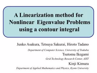
1 / 31
310 likes | 519 Views
Nonlinear. A Linearization method for Polynomial Eigenvalue Problems using a contour integral . Junko Asakura , Tetsuya Sakurai , Hiroto Tadano Department of Computer Science, University of Tsukuba Tsutomu Ikegami Grid Technology Research Center, AIST Kinji Kimura

E N D
Nonlinear A Linearization method for Polynomial Eigenvalue Problems using a contour integral Junko Asakura, Tetsuya Sakurai, Hiroto Tadano Department of Computer Science, University of TsukubaTsutomu Ikegami Grid Technology Research Center, AIST Kinji Kimura Department of Applied Mathematics and Physics, Kyoto University
Outline • Background • Linearization method for PEPs using a contour integral • Extension to analytic functions • Numerical Examples • Conclusions A linearization method for PEPs IWASEP7, Dubrovnik
Background A linearization method for PEPs IWASEP7, Dubrovnik
Polynomial Eigenvalue Problems F(z)x= 0 • Oscillation analysis with damping • Stability problems in fluid dynamics • 3D-Schrödinger equation etc F(z) = zlAl+ zl-1Al-1 + ・・・ +zA1 + A0 Ak Applications: Eigenvalues in a specified domain are required in some applications A linearization method for PEPs IWASEP7, Dubrovnik
Projection method for generalized eigenvalue problems using a contour integral Sakurai-Sugiura(SS) method [1] Ax = Bx [1] Sakurai, T., Sugiura, H., A projection method for generalized eigenvalue problems. J. Comput. Appl. Math. 159( 2003)119-128 A linearization method for PEPs IWASEP7, Dubrovnik
Linearization method for polynomial eigenvalue problems using a contour integral A linearization method for PEPs IWASEP7, Dubrovnik
The eigenvalues of the pencil (H< , Hm) are given by 1, …, m. m Sakurai-Sugiura method :a positively oriented closed Jordan curve (j, uj) :eigenpairs of the matrix pencil(A, B) in Γ (j=1,..., m) v : an arbitrary nonzero vector A linearization method for PEPs IWASEP7, Dubrovnik
Modification of the moments k for PEPs :a positively oriented closed Jordan curve (j, uj) :eigenpairs of the matrix pencil(A, B) in Γ (j=1,..., m) A linearization method for PEPs IWASEP7, Dubrovnik
Modification of the moments kfor PEPs F(z) = zlAl+ zl-1Al-1 + ・・・ +zA1 + A0 Ak A linearization method for PEPs IWASEP7, Dubrovnik
The eigenvalues of the pencil are given by 1, …, m The Main Theorem F(z): a regular polynomial matrix 1, …, m: simple eigenvalues of F(z) in A linearization method for PEPs IWASEP7, Dubrovnik
The Smith Form F(z) : n × n regular matrix polynomial F(z) admits the representation P(z)F(z)Q(z) = D(z) where D(z) = . di:monic scalar polynomials s.t. di is divisible by di-1 P(z), Q(z): n×n matrix polynomials with constant nonzero determinants A linearization method for PEPs IWASEP7, Dubrovnik
, , F(z): a regular polynomial matrix 1, …, m: simple eigenvalues of F(z) in P(z)F(z)Q(z) = D(z): The Smith Form of F(z) A linearization method for PEPs IWASEP7, Dubrovnik
Linearization method for polynomial eigenvalue problems using a contour integral Polynomial Eigenvalue Problem F(z)x = 0 F(z) = zlAl+ zl-1Al-1 + ・・・ +zA1 + A0 Generalized Eigenvalue Problem H<x = Hmx H< = [i+j-2]i, j=1, Hm = [i+j-1]i, j=1 m m m m A linearization method for PEPs IWASEP7, Dubrovnik
Extension into Analytic Functions F(z)x= 0 fij: an analytic function in , i, j= 1, …, n A linearization method for PEPs IWASEP7, Dubrovnik
Elementary transformations (1) Interchange two rows (2) Add to some row another row multiplied by an analytic function inside and on the given domain (3) Multiply a row by a nonzero complex number together with the three corresponding operations on columns. A linearization method for PEPs IWASEP7, Dubrovnik
the Smith Form for Nonlinear Eigenvalue Problem F(z) : n × n regular matrix F(z) admits the representation P(z)F(z)Q(z) = D(z) where D(z) = di: analytic function inside and on such that di is divisible by di-1, i=1, …, n-1 P(z), Q(z): n×n matrix with constant nonzero determinants A linearization method for PEPs IWASEP7, Dubrovnik
:a positively oriented closed Jordan curve (j, uj) :eigenpairs of the matrix polynomial F(z) in Γ (j=1,..., m) V : a regular matrix , Block version of the Sakurai-Sugiura method Block SS method[2] [2] T. Ikegami, T. Sakurai, U. Nagashima, A filter diagonalization for generalized eigenvalue problems based on the Sakurai-Sugiura method (submitted) A linearization method for PEPs IWASEP7, Dubrovnik
V , det(V) ≠ 0 Computation of Mk Approximate the integral of k via N-point trapezoidal rule: , k = 0, …, 2m-1 j := + exp(2i/N(j+1/2)), j = 0, …, N-1 A linearization method for PEPs IWASEP7, Dubrovnik
xj:eigenvectors of the pencil (H<, Hm) m Computation of the eigenvectors of F(z) The eigenvectors of F(z) are computed by qn(j) = jSxj, j≠ 0 where S = [s0, …, sk], k=0, …, m-1 A linearization method for PEPs IWASEP7, Dubrovnik
Algorithm: Block SS method Input: F(z), V , N, M, , Output: 1, …, K, qn(1), …, qn(K) Set j ← + exp(2i/N(j+1/2)), j = 0, …, N-1 Compute VHF(j)-1V, j = 0,…, N-1 Compute Mk, k = 0, …, 2m-1 Construct Hankel matrices Compute the eigenvalues 1, …, K of Compute qn(1), …, qn(K) Set j = + j, j = 1, ..., K A linearization method for PEPs IWASEP7, Dubrovnik
Numerical Examples A linearization method for PEPs IWASEP7, Dubrovnik
Numerical Examples Test Problems • Example1: Quadratic Eigenvalue Problem • Example2: Eigenvalue Problem for a Matrix whose elements are Analytic Functions • Example3: Quartic Eigenvalue Problem Test Environment • MacBook Core2Duo 2.0GHz • Memory 2.0Gbytes • MATLAB 7.4.0 A linearization method for PEPs IWASEP7, Dubrovnik
Test Matrix: Eigenvalues: 1/3, 1/2, 1, i, -i, ∞ Parameters: Γ= ei| 0≦q≦2 } γ = 0, L = 1 Example1 Im eigenvalue × × × × Re × 5 eigenvalues lie in A linearization method for PEPs IWASEP7, Dubrovnik
:result, :exact Results of Example1 A linearization method for PEPs IWASEP7, Dubrovnik
Equivalent to Example2 Test matrix: Eigenvalues: 0, /2, -/2, , -log7(≒1.9459) ≦z≦) Parameters: Γ= ei| 0≦q≦2 } γ = 0, 3.2 L = 2 A linearization method for PEPs IWASEP7, Dubrovnik
:result, :exact Results of Example2 A linearization method for PEPs IWASEP7, Dubrovnik
Ai , i = 0, 1, 2, 3, 4 Example3 Test Matrix: Quartic Matrix Polynomial “butterfly” in NLEVP[3] F(z) = 4A4+3A3+2A2+A1+A0 [3] T. Betcke, N. J. Higham, V. Mehrmann, C. Schröder, and F. Tisseur, NLEVP: A Collection of Nonlinear Eigenvalue Problems, MIMS EPrint 2008.40 (2008) A linearization method for PEPs IWASEP7, Dubrovnik
→ Example3 Parameters: Γ= ei| 0≦q≦2 } γ = 1-i, L = 24 A total of 13 eigenvalues lie in A linearization method for PEPs IWASEP7, Dubrovnik
Results of Example3 +: results of “polyeig” o: results of the proposed method max residual of eigenvalues calculated by the proposed method: 7.40e-12 → A linearization method for PEPs IWASEP7, Dubrovnik
Conclusions A linearization method for PEPs IWASEP7, Dubrovnik
Conclusions Summary of Our Study • We proposed a linearization method for PEPs using a contour integral. • We extended the proposed method to nonlinear eigenvalue problems. Future Study • Precise theoretical observation of the extension to nonlinear eigenvalue problems • Estimation of suitable parameters A linearization method for PEPs IWASEP7, Dubrovnik